Chapter 5 Instruction Sets and Addressing Modes
Chapter 5 Instruction Sets and Addressing Modes. Chapter 5 Objectives. Understand the factors involved in instruction set architecture design. Gain familiarity with memory addressing modes. Understand the concepts of instruction-level pipelining and its affect upon execution performance.

Chapter 5 Instruction Sets and Addressing Modes
E N D
Presentation Transcript
Chapter 5 Instruction Sets and Addressing Modes
Chapter 5 Objectives • Understand the factors involved in instruction set architecture design. • Gain familiarity with memory addressing modes. • Understand the concepts of instruction-level pipelining and its affect upon execution performance.
5.2 Instruction Formats • Instruction set is the collection of instructions that a CPU can execute • They are differentiated by the following: • Number of bits per instruction. • Stack-based or register-based. • Number of explicit operands per instruction. • Operand location. • Types of operations. • Type and size of operands. • Type of addressing modes • Number of registers 3
5.2 Instruction Formats • Other major architectural considerations are: • Memory organization (byte- or word-addressable) • Byte ordering or endianness • Endianness • If we have a two-byte integer, the integer may be stored so that the least significant byte is followed by the most significant byte or vice versa. • In little endian machines,the least significant byte is followed by the most significant byte. • Big endian machines store the most significant byte first (at the lower address). 4
5.2 Instruction Formats • As an example, suppose we have the hexadecimal number 12345678. • The big endian and small endian arrangements of the bytes are shown below. • Important for a program or software application that writes/reads data to a file. • Adobe Photoshop uses big endian, PDF is little endian. 5
5.2 Instruction Formats • Big endian: • Is more natural (easier to read dumps) • The sign of the number can be determined by looking at the byte at address offset 0. • Strings and integers are stored in the same order. • Little endian: • Makes it easier to place values on non-word boundaries. • It does not require to begin on even-numbered byte address • Conversion from a 16-bit integer address to a 32-bit integer address does not require any arithmetic. 6
5.2 Instruction Formats • The next consideration for architecture design concerns how the CPU will store data. • We have three choices: 1. A stack architecture 2. An accumulator architecture 3. A general purpose register architecture. • In choosing one over the other, the tradeoffs are simplicity (and cost) of hardware design with execution speed and ease of use. 7
5.2 Instruction Formats • In a stack architecture, • Stack implicitly keeps instructions and operands. • A stack cannot be accessed randomly. • In an accumulator architecture, • one operand of a binary operation is implicitly in the accumulator. • One operand is in memory, creating lots of bus traffic. • In a general purpose register (GPR) architecture, • Registers can be used instead of memory. • Faster than accumulator architecture. • Good if memory is slow • Efficient implementation for compilers. 8
5.2 Instruction Formats • Most systems today are GPR systems w/three types: • Memory-memory where two or three operands may be in memory. • Register-memory where at least one operand must be in a register. • Load-store where no operands may be in memory. • Instruction length depends on the # of operands and the # of available registers. Two types: • Fixed length: wastes space but better for pipelining • Variable length: more complex but saves space • Instruction format: OPCODE + (0|1|2|3) addresses 9
5.2 Instruction Formats • Stack machines • They use one - and zero-operand instructions. • LOAD and STORE instructions require a single memory address operand. • Other instructions use operands from the stack implicitly. • PUSH and POP operations involve only the stack’s top element. • Binary instructions (e.g., ADD, MULT) use the top two items on the stack. • Stack architectures require us to think about arithmetic expressions a little differently. 10
5.2 Instruction Formats • Arithmetic expressions using infix notation, such as: Z = X + Y. • Stack arithmetic requires that we use postfix notation: Z = XY+. • This is also called reverse Polish notation, in honor of its Polish inventor, Jan Lukasiewicz (1878 – 1956). • The principal advantage of postfix notation is that parentheses are not used. • Infix expression:Z = (X Y) + (W U), • Becomes: Z = X Y W U + (in postfix notation) 11
5.2 Instruction Formats • In a stack ISA, the postfix expression, Z = X Y W U + might look like this: PUSH X PUSH Y MULT PUSH W PUSH U MULT ADD POP Z Note: The result of a binary operation is implicitly stored on the top of the stack! 12
5.2 Instruction Formats • In a one-address ISA, like MARIE, the infix expression, Z = X Y + W U looks like this: LOAD X MULT Y STORE TEMP LOAD W MULT U ADD TEMP STORE Z 13
5.2 Instruction Formats • In a two-address ISA, (e.g.,Intel, Motorola), the infix expression, Z = X Y + W U might look like this: LOAD R1,X MULT R1,Y LOAD R2,W MULT R2,U ADD R1,R2 STORE Z,R1 Note: Two-address ISAs usually require one operand to be a register. 14
5.2 Instruction Formats • With a three-address ISA, (e.g.,mainframes), the infix expression, Z = X Y + W U might look like this: MULT R1,X,Y MULT R2,W,U ADD Z,R1,R2 Would this program execute faster than the corresponding (longer) program that we saw in the stack-based ISA? 15
5.2 Instruction Formats • Design issues • Instructions with more addresses • More complex • Fewer instructions per program • Instruction with fewer addresses • Less complex • Faster fetch/decode/execution of instructions • More instruction per program
5.2 Instruction Formats • We have seen how instruction length is affected by the number of operands supported by the ISA. • In any instruction set, not all instructions require the same number of operands. • Operations that require no operands, such as HALT, necessarily waste some space when fixed-length instructions are used. • One way to recover some of this space is to use expanding opcodes. 17
5.2 Instruction Formats • Expanding opcodes: • A system has 16 registers and 4K of memory. • We need 4 bits to access one of the registers. We also need 12 bits for a memory address. • If the system is to have 16-bit instructions, we have two choices for our instructions: 18
5.2 Instruction Formats • If we allow the length of the opcode to vary, we could create a very rich instruction set: Decoding is more complex! 19
5.3 Instruction types Instructions fall into several broad categories that you should be familiar with: • Data movement. • Arithmetic operations. • Boolean. • Bit manipulation. • I/O. • Control transfer. • Special purpose. Can you think of some examples of each of these? 20
5.4 Addressing • Addressing modes specify where an operand is located. • They can specify a constant, a register, or a memory location. • The actual location of an operand is its effective address (EA). • Certain addressing modes allow us to determine the address of an operand dynamically. 21
5.4 Addressing • Immediate addressing is where the data is part of the instruction. • e.g., ADD 5 ==> add 5 to AC, 5 is the operand • Advantage: Fast, no memory reference • Disadvantage: Limited range (for constant) • Direct addressing is where the address of the data is given in the instruction. • ADD A ==> Add content of memory location pointed A to AC • Advantage: No additional calculation to find EA, EA=A • Disadvantage: Limited address space. 22
5.4 Addressing • Register addressing is where the data is located in a register. • Similar to direct addressing, EA = R • e.g., ADD R3 ==> add content of register 3 to AC • Advantage: small address field needed, faster instruction execution, no memory access • Disadvantage: limited number of registers, programmers must use them efficiently • Indirect addressing gives the address of the address of the data in the instruction. • Advantage: large address space and maybe nested • Disadvantage: multiple memory accesses (slower)
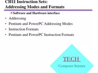
Instruction Opcode Register Address R Memory Registers Pointer to Operand Operand 5.4 Addressing • Register indirect addressing uses a register to store the address of the address of the data. • Analogous to indirect addressing • Register holds address of operand, EA = (R) • e.g., ADD (R3) • Advantage: larger address space • Disadvantage: Multiple references to reach the operand
5.4 Addressing • Displacement Addressing • It combines direct- with register indirect addressing • EA = A + (R) • Instruction must hold two addresses • Three common use of displacement addressing • Relative addressing • EA = A + (PC) • Good for locality of reference and cache usage • Indexed addressing • Based addressing
5.4 Addressing • Indexed addressing • A holds base address, R holds displacement • Good for accessing arrays • Based addressing • A holds displacement, R holds pointer to base register • R may be explicit or implicit (segment-based register) • Main difference between these two is that: • an index register holds an offset relative to the address given in the instruction, a base register holds a base address where the address field represents a displacement from this base. 26
5.4 Addressing • In stack addressing the operand is assumed to be on top of the stack. • There are many variations to these addressing modes including: • Postindex: Indexing performed after indirection • EA = (A) + (R) • Preindex: Indexing performed before indirection • EA = (A + (R)) • Auto increment, -decrement: • Special cases of based addressing • EA = (R)++ or --(R) 27
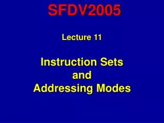
Instruction Opcode Register R A Memory Registers Displacement Operand + 5.4 Addressing • Preindex addressing • Good for implementing a multiway branch • Postindex addressing • Good for accessing one of a number of blocks Instruction Opcode Register R A Memory Registers + Operand
5.4 Addressing • These are the values loaded into the accumulator for each addressing mode for the instruction below. 29
Intel Architecture: IA-32 Pentium • Implemented on Pentium processors • Memory is byte-addressable using 32-bit addresses • Registers: • Eight 32-bit general-purpose (R0-R7), • Eight floating points holding doubleword or quadword operands, • Segments: code (CS), four data (DS, ES, FS, GS), and stack (SS) • Instruction pointer and status register • IA-32 general-purpose registers allow for compatibility with earlier Intel processors • R0-R7 correspond to extended registers: EAX, ECX, EDX, EBX, ESP, EBP, ESI, EDI • They are extended versions of the corresponding 16-bit registers (AX, CX, …) of earlier processors.
Pentium addressing modes • Effective address (EA) of an operand is computed as: EA = B + ( I*S ) + D • B: base register • I: index register • S: scale • D: displacement • EA is an offset into a segment • When ESP or EBP is used as a base register, the SS segment is the default segment.
Pentium addressing modes (cont.) • Modes: • Immediate mode: Operand = Value (value is a signed #) • Example: MOV ECX, 20 20 is copied into ECX • Register direct mode: EA = B • Example: ADD EAX, EDX Add contents of EDX and EAX • Direct mode: EA = location (location is a 32-bit address) • Example: MOVE SUM, EAX Move EAX content into SUM
Pentium addressing modes (cont.) • Register indirect mode: EA = [B] • Example: MOV EAX, [EBX] • Base with displacement mode: EA = [B] + displacement • Example: MOV EAX, [EBP + 10] • Index with displacement mode: EA = [I]*S + displacement • e.g., ADD EAX, [4*ESI+10] • Base with index mode: EA = [B] + [I]*S • Example: MOV EAX, [ESP + ESI] • Base with index and displacement mode: • EA = [B] + [I]*S + displacement • Example: ADD EDI, [EBX + 4*ESI + 120] • PC relative mode: EA = [PC] + value (e.g., JMP Loop)
Pentium instruction format (cont.) • An instruction can range from 1 byte (opcode) to 11 or more • INC EDI 47h opcode reg:EAX • ADD EAX, 10 03h | 00 000 101| A : 03050000000Ah MOD R/M : 05h32-bit displacement • ADD EAX, [EBX + EDI*4] 0304BBh Opcode MOD R/M Scale index base MOD R/M: 00100 means an SIB follows ([ ][ ]) 03h 00 000 100 10 111 011
MIPS Architecture • Addressing modes • Immediate mode • Register mode • Base with displacement mode • PC-relative mode • PC-pseudodirect mode • Used in the jump address • Address is the 26 bits of the instruction “+” the upper bits of the PC • Hardware has 32 registers, 32-bit wide each • Use two-character names following a dollar sign ($t0, $s1) • Register 0 is named $zero holding a constant zero • Registers 8-15 are named $t0 - $t7 (used for temporary storage) • Registers 16-23 are named $s0 - $s7 (used to save values)
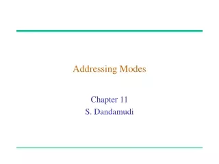
From the low order 16 bits of the branch instruction (PC-relative addressing) 16 offset sign-extend 00 ? branch dst address 32 32 Add PC 32 32 Add 32 4 32 32 From the low order 26 bits of the jump instruction (PC-pseudo addressing) 26 00 32 4 PC 32 MIPS: Addressing modes
MIPS: Instruction formats • R-format: | op | rs | rt | rd | shamt | funct | 6 bits 5 bits 5 bits 5 bits 5 bits 6 bits • op (operation), rs (first register source operand), rt (second register source operand), rd (register destination operand), shamt (shift amount), funct (function or variant of the operation) • Example: add $t0, $s1, $s2 meaning $t0 = $s1 + $s2 Where $t0 = 8, $s1 = 17, $s2 = 18, op(add) = 0, funct = 32 | 000000 | 10001 | 10010 | 01000 | 00000 | 100000 | • I-format: | op | rs | rt | immediate | 6 bits 5 bits 5 bits 16 bits • Example: Load A[8] in register $t0, where A[0] is pointed by $s3 • lw $t0, 32($s3) | 100011 | 10011 | 01000 | 0000000000100000 | • J-format: | op | jump address | 6 bits 26 bits • Used by the unconditional jump instruction: j label
5.5 Instruction-Level Pipelining • Some CPUs divide the fetch-decode-execute cycle into smaller steps. • These smaller steps can often be executed in parallel to increase throughput. • Such parallel execution is called instruction-level pipelining. • This term is sometimes abbreviated ILP in the literature. The next slide shows an example of instruction-level pipelining. 41
5.5 Instruction-Level Pipelining • Suppose a fetch-decode-execute cycle were broken into the following smaller steps: • Suppose we have a six-stage pipeline. S1 fetches the instruction, S2 decodes it, S3 determines the address of the operands, S4 fetches them, S5 executes the instruction, and S6 stores the result. 1. Fetch instruction. 4. Fetch operands. 2. Decode opcode. 5. Execute instruction. 3. Calculate effective 6. Store result. address of operands. 42
5.5 Instruction-Level Pipelining • For every clock cycle, one small step is carried out, and the stages are overlapped. S1. Fetch instruction. S4. Fetch operands. S2. Decode opcode. S5. Execute. S3. Calculate effective S6. Store result. address of operands. 43
5.5 Instruction-Level Pipelining • The theoretical speedup offered by a pipeline can be determined as follows: Let tp be the time per stage. Each instruction represents a task, T, in the pipeline. The first task (instruction) requires ktp time to complete in a k-stage pipeline. The remaining (n - 1) tasks emerge from the pipeline one per cycle. So the total time to complete the remaining tasks is (n - 1)tp. Thus, to complete n tasks using a k-stage pipeline requires: (ktp) + (n - 1)tp = (k + n - 1)tp. 44
5.5 Instruction-Level Pipelining • If we take the time required to complete n tasks without a pipeline and divide it by the time it takes to complete n tasks using a pipeline, we find: • If we take the limit as n approaches infinity, (k + n - 1) approaches n, which results in a theoretical speedup of: 45
5.5 Instruction-Level Pipelining • Our neat equations take a number of things for granted. • First, we have to assume that the architecture supports fetching instructions and data in parallel. • Second, we assume that the pipeline can be kept filled at all times. This is not always the case. Pipeline hazards arise that cause pipeline conflicts and stalls. 46
5.5 Instruction-Level Pipelining • An instruction pipeline may stall, or be flushed for any of the following reasons: • Resource conflicts. • Access memory at the same time by different stages • Data dependencies. • Example: add R0, R3, R1 <== R0=R3+R1 sub R2, R0, R3 <== it uses R0 • Conditional branching. • Branching invalidates several instructions in the pipeline ( pipeline must be cleared and restarted) 47
Examples of systems with pipelining • We return briefly to the Intel and MIPS architectures from the last chapter, using some of the ideas introduced in this chapter. • Intel introduced pipelining to their processor line with its Pentium chip. • The first Pentium had two five-stage pipelines. Each subsequent Pentium processor had a longer pipeline than its predecessor with the Pentium IV having a 24-stage pipeline. • The Itanium (IA-64) has only a 10-stage pipeline. 48
Examples of systems with pipelining • MIPS was an acronym for Microprocessor Without Interlocked Pipeline Stages. • The architecture is little endian and word-addressable with three-address, fixed-length instructions. • Like Intel, the pipeline size of the MIPS processors has grown: The R2000 and R3000 have five-stage pipelines.; the R4000 and R4400 have 8-stage pipelines. 49
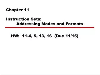
Pipeline MIPS http://en.wikipedia.org/wiki/Image:Pipeline_MIPS.png Controls & Buffers