Window Quick Tips:
Window Quick Tips:. hold down CTRL and spin the mouse wheel to zoom in and out hold down the ALT key and tap the TAB key to flip between open programs (like the last channel button on TV). Microsoft Excel: Cells, Columns and Rows. Cells (the little boxes in excel) Hold numbers or text

Window Quick Tips:
E N D
Presentation Transcript
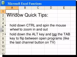
Window Quick Tips: • hold down CTRL and spin the mouse wheel to zoom in and out • hold down the ALT key and tap the TAB key to flip between open programs (like the last channel button on TV)
Microsoft Excel:Cells, Columns and Rows • Cells (the little boxes in excel) • Hold numbers or text • Contents viewed on edit line • Named like battleship – column and row. Cell A6 is named for where column A meets row 6
Excel Formulas • Excel can be used as a big calculator • Basic arithmetic (+, -, x , ÷ and yx) • Operation symbols: Subtraction: - Addition: + Multiplication: * Division: / Exponent: ^
Formulas Using Numbers • Syntax: always begins with equals sign • Example1 : seven times eight • Choose a cell and type =7*8 • When you hit enter the number 56 will appear • Example 2: four to the third power • Choose a cell and =4^3 • When you hit enter the number 64 will appear
Formulas Using Cell Names • you can use cell names as variables • Example1: Seven times the value in cell B2 • Type =7*B2 (cell B2 will be automatically outlined) • Example2: the value in cell B2 plus the value in cell B5 • Type =B2+B5 (both cells will be outlined)
Try this out…. • In cell B2 create a formula to multiply the values of cells B5 and B7 and divide by 4. • =B5*B7/4 answer should be zero • Add numbers to cells B5 and B7
Excel Functions • Excel Functions do many things from calculating an average to finding standard deviation to combining several lines of text.
Excel Functions • Excel functions ALWAYS begin with an equals sign: • Form of an Excel function is: =function_name(argument1,argument2… ) Arguments are additional pieces of information Excel needs to do what you are asking it to do Arguments are always separated by commas.
sum=sum(number/cell_names) • Function sum has one or more arguments • number are actual numbers separated by commas • cell names are individual cell references separated by a comma or a range of cells. A range is shown using the first and last cell in the range separated by a colon.
sum using the autosum button • button showing Σ(greek letter sigma) automatically sums up the nearest range of numbers it can find. • The range must be continuous (no empty cells) for Excel to automatically choose the correct data
round=round(number,num_digits) • Function round has two arguments • Number is a number or cell value you want rounded • Num_digits is the number of digits you want rounded to. Zero and negative numbers will round to whole number place values. (0 round to ones, -1 rounds to tens, -2 rounds to hundreds, etc.)
average=average(range of cells) • Average function has one argument: a range of cells with numbers you want to average • It is on the pull-down menu attached to the autosum button • Simple as autosum – just select the range you want and hit enter
median=median(range of cells) • Median function has one argument: a range of cells with a dataset from which you want to determine the median • It is NOT on the pull-down menu attached to the autosum button • Can type it in as above or use More Functions from the autosum pull-down • Could also use insert function: fx
mode=mode(range of cells) • Mode function has one argument: a range of cells with a dataset from which you want to determine the median • It is NOT on the pull-down menu attached to the autosum button • Can type it in as above or use More Functions from the autosum pull-down • Could also use insert function: fx
mode(continued) • Mode will return the number that appears most often in a data set. • If there is no mode (no repeating numbers) Excel will show #N/A • Warning: If there is a bimodal set of data Excel will show the mode of the first repeating number in the set….
mode(continued) • If your data is as follows: • The numbers 2 and 3 are both modes: they both appear twice but Excel shows only 2 since it appears first in the data • Why? IDK, blame Excel.
rangethere is no range function • There is no one function that can get you the range of a dataset. You must: • Use several cells with functions to calculate it OR • Combine several functions into a single cell to find it • The simplest way is to subtract a =min function from a =max function: • =max(B2:B6)-min(B2:B6) (no equals sign for the 2nd one)
Logical Functions • Logical functions make decisions about information in a cell based on conditions you set and answer by displaying info depending on the decision • Conditions – criteria you set for Excel • (i.e. is the cell =5, is the cell >14, etc.)
if=if(logical test, value if true, value if false) • If function has three arguments: • 1. a logical test seeing if something is true or false in a cell • 2. a value that shows up if the logical test is true • 3. a value to show up if the logical test if false
if(cont)=if(logical test, value if true, value if false) • Argument 1: logical test • For the logical test argument you put a cell reference and a condition • i.e. you want to see if cell B2 is equal to 5. The first part of the function looks like this: =if(B2=5,
if(cont)=if(logical test, value if true, value if false) • Argument 2: value if true • For value if true argument you put a number or text for Excel to show if the logical test turns out to be true • i.e. if cell B2 actually equal to 5 let’s say you want the word EQUAL appear. The second part of the function looks like this: =if(B2=5,”EQUAL”, (remember, all text must be enclosed in double quotes)
if(cont)=if(logical test, value if true, value if false) • Argument 3: value if false • For value if false argument you put a number or text for Excel to show if the logical test turns out to be false • i.e. if cell B2 does NOT equal to 5 let’s say you want the word NOT EQUAL appear. The last part of the function looks like this: =if(B2=5,”EQUAL”,”NOT EQUAL”) (remember, all text must be enclosed in double quotes)
if(cont)=if(logical test, value if true, value if false) So if we take our example it looks like this:
if(cont)=if(logical test, value if true, value if false) Hitting enter gives us the function result which is EQUAL since cell B2=5
if(cont)=if(logical test, value if true, value if false) If we change the value in cell B2 to 8 it gives us the function result which is NOT EQUAL since cell B2 is no longer equal to 5
Text Functions • Functions you can use to manipulate text in a bunch of ways • UPPER function • LOWER function • PROPER function • CONCATENATE function
upper=upper(text) • Function has one argument • Converts text to all upper case letters • Text is typed words/numbers OR the cell that contains typed words/numbers
lower=lower(text) • Function has one argument • Converts text to all lower case letters • Text is typed words/numbers OR the cell that contains typed words/numbers
proper=proper(text) • Function has one argument • Converts text to all first letters upper case and all the rest lower case • Text is typed words/numbers OR the cell that contains typed words/numbers
concatenate=concatenate(text1, text2…) • Function has several argument • Combines text from multiple cells into one cell • The arguments are cells with text OR text in double quotation marks
Lookup Functions • Excel can be used to look up information in a table, similar to looking in a dictionary or phone book • A table is a list of data, each column having its own unique info or field
vlookup=vlookup(lookup_value,table_array,column_number)) • lookup_value : a cell where you will type the data that you want to seek on a table • i.e. in the database below I want to type a name in cell A2 to get more info from the table
vlookup=vlookup(lookup_value,table_array,column_number)) • table_array : information arranged in columns and rows • i.e. the table that the vlookup function goes to find the info in cell A2
vlookup=vlookup(lookup_value,table_array,column_number)) • column_number : column in the table that you want excel to return • i.e. column 2 will make vlookup send the phone number back into the function’s cell
Font Formatting • Everything is the same as Word: font, color, size, bold, italic, underline EXCEPT Formatting Borders around cells
Border Formatting • Found on the Font section of the Home ribbon. • Can make a variety of borders around single cells or groups of cells
Border Formatting • Pre set border selections appear on the pull-down menu while a box with custom settings can be found by clicking More Borders on the bottom
Alignment Formatting • Allows you to line up text within a cell to the left, right or center (like Word) • Also allows you to align text vertically within the cell – on the top, center, or bottom
Alignment Formatting • Examples:
Number Formatting • Currency • shows numbers with two decimals and a currency symbol of your choosing (dollars $, pounds ₤, yen ¥, euros €) • On a pull-down menu off the
Number Formatting • Fraction • shows numbers as fractions or mixed numbers • On the pull-down menu • You set the number of digits for the denominator
Number Formatting • Fraction (cont) • Mixed numbers are entered by typing the whole number, then a space, then a fraction. • Mathematical operations can be done on cells formatted for fraction • The answers will appear as fractions
Number Formatting • Scientific Notation • shows large or small numbers with a base and power using the letter E to show exponent/power i.e. – 4.7 x 10³ becomes 4.7E+3 meaning 4.7 raised to the +3 power