Inference about Comparing Two Populations
820 likes | 981 Vues
Inference about Comparing Two Populations. Chapter 13. 13.1 Introduction.

Inference about Comparing Two Populations
E N D
Presentation Transcript
Inference about Comparing Two Populations Chapter 13
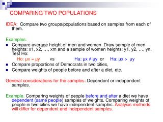
13.1 Introduction • In previous discussions we presented methods designed to make an inference about characteristics of a single population. We estimated, for example the population mean, or hypothesized on the value of the standard deviation. • However, in the real world we encounter many times the need to study the relationship between two populations. For example: • We want to compare the effects of a new drug on blood pressure, in which case we can test the relationship between the mean blood pressure of two groups of individuals: those who take the drug, and those who don’t. • We are interested in the effects a certain ad has on voters’ preferences as part of an election campaign. In this case we can estimate the difference in the proportion of voters who prefer one candidate before and after the ad is televised.
13.1 Introduction • Variety of techniques are presented whose objective is to compare two populations. • These techniques are designed to compare: • two population means. • two population variances. • two proportions.
The reason we are looking at the difference between the two means is that is strongly related to a normal distribution, whose mean is m1 – m2. See next for details. • Two random samples are therefore drawn from the two populations of interest and their means and are calculated. 13.2 Inference about the Difference between Two Means: Independent Samples • We’ll look at the relationship between the two population means by analyzing the value of m1 – m2.
The Sampling Distribution of • is normally distributed if the (original) population distributions are normal . • is approximately normally distributed if the (original) population is not normal, but the samples’ size is sufficiently large (greater than 30). • The mean value of is m1 - m2 • The variance of is
Making an inference about m1– m2 • The Z – score of is • However, if is normal or approximately normal, then Z is standard normal. So… • Z can be used to build a confidence interval or test a hypothesis about m1-m2. See next.
Making an inference about m1– m2 • Practically, the “Z” statistic is hardly used, because the population variances are not known. • Instead, we construct a “t” statistic using the • sample “variances” (and ). t S22 S12 ? ?
Making an inference about m1– m2 • Two cases are considered when producing the t-statistic. • The two unknown population variances are equal. • The two unknown population variances are not equal.
Inference about m1– m2: Equal variances • If the two variances and are equal to one another, then and estimate the same value. • Therefore, we can pool the two sample variances and provide a better estimate of the common populations’ variance, based on a larger amount of information. • This is done by forming the pooled variance estimate. See next.
To get some intuition about this pooled estimate,note that we can re-write it as which has the form of a weighted average of the two sample variances. The weights are the relative sample sizes. A larger sample provides larger weight and thus influences the pooled estimate more (it might be easier to eliminate the values ‘-1’ and ‘-2’ from the formula in order to see the structuremore easily. Inference about m1– m2: Equal variances • Calculate the pooled variance estimate by:
Example: S12 = 25; S22 = 30; n1 = 10; n2 = 15. Then, Inference about m1– m2: Equal variances • Calculate the pooled variance estimate by:
Note how Sp2 replaces bothS12 and S22. Inference about m1– m2: Equal variances • Construct the t-statistic as follows:
Inference about m1– m2: Unequal variances • Since and are unequal • we can’t produce a single estimate • for both variances. • Thus we use the sample variances in the ‘t’ formula
Which case to use:Equal variance or unequal variance? • Whenever there is insufficient evidence that the variances are unequal, it is preferable to run the equal variances t-test. • This is so, because for any two given samples The number of degrees of freedom for the equal variances case The number of degrees of freedom for the unequal variances case ³
Example: Making an inference about m1– m2 • Example1 • Do people who eat high-fiber cereal for breakfast consume, on average, fewer calories for lunch than people who do not eat high-fiber cereal for breakfast? • A sample of 150 people was randomly drawn. Each person was identified as a consumer or a non-consumer of high-fiber cereal. • For each person the number of calories consumed at lunch was recorded.
Example: Making an inference about m1– m2 • Solution: • The data are quantitative. • The parameter to be tested is • the difference between two means. • The claim to be tested is: • The mean caloric intake of consumers (m1) • is less than that of non-consumers (m2).
Example: Making an inference about m1– m2 • The hypotheses are: • H0: m1 - m2 = 0 • H1: m1 - m2 < 0 • To check the relationships between the variances, we use a computer output to find the sample variances (Xm13-1.xlsx). From the data we have S12= 4103, and S22 = 10,670. • It appears that the variances are unequal. m1= mean caloric intake for fiber consumers m2= mean caloric intake for fiber non-consumers
Example: Making an inference about m1– m2 • Solving by hand • From the data we have:
Example: Making an inference about m1– m2 • Solving by hand • H1: m1 - m2 < 0The rejection region is t < -ta,df = -t.05,123 @ -1.658
The p-value approach: .01929 < .05 The rejection region approach-2.09107 < -1.65734 Example: Making an inference about m1– m2 Conclusion: At 5% significance level there is sufficient evidence to reject the null hypothesis, and argue thatm1 < m2. Click.
Example: Making an inference about m1– m2 • Solving by hand The confidence interval estimator for the differencebetween two means when the variances are unequal is
Example: Making an inference about m1–m2 Note that the confidence interval for the differencebetween the two means falls entirely in the negativeregion: [-56.86, -1.56]; even at best the difference between the two means is m1 – m2 = -1.56, so we can be 95% confident m1 is smaller than m2! This conclusion agrees with the results of the test performed before.
Example: Making an inference about m1– m2 • Example 2 • An ergonomic chair can be assembled using two different sets of operations (Method A and Method B) • The operations manager would like to know whether the assembly time under the two methods differ.
Example: Making an inference about m1– m2 • Example 13.2 • Two samples are randomly and independently selected • A sample of 25 workers assembled the chair using design A. • A sample of 25 workers assembled the chair using design B. • The assembly times were recorded • Do the assembly times of the two methods differs?
Example: Making an inference about m1– m2 Assembly times in Minutes • Solution • The data are quantitative. • The parameter of interest is the difference • between two population means. • The claim to be tested is whether a difference • between the two designs exists.
Example: Making an inference about m1– m2 • Solving by hand • The hypotheses test is: • H0: m1 - m2= 0 H1: m1 - m2¹ 0 • Since we ask whether or not the assembly times are the same on the average, the alternative hypothesis is of the form m1¹ m2 • To check the relationship between the two variances we run the F test. (Xm13-02). • From the data we have = 0.8478, and =1.3031.The p-value of the F test = 2(.1496) = .299 • Conclusion: s12 and s22 appear to be equal.
Example: Making an inference about m1– m2 • Solving by hand • To calculate the t-statistic we have:
Rejection region Rejection region Example: Making an inference about m1– m2 • The 2-tail rejection region is t < -ta/2,n =-t.025,48 = -2.009 or t > ta/2,n = t.025,48 = 2.009 • The test: Since t= -2.009 < 0.93 < 2.009, there is insufficient evidence to reject the null hypothesis. For a = 0.05 .093 2.009 -2.009
-2.0106 < .9273 < +2.0106 .35839 > .05 Example: Making an inference about m1– m2 Conclusion: From this experiment, it isunclear at 5% significance level if the two assembly methods are different in terms of assembly time
Example: Making an inference about m1– m2: A 95% confidence interval for m1 - m2 when the two variances areequal is calculated as follows: Thus, at 95% confidence level -0.3176 < m1 - m2 < 0.8616 Notice: “Zero” is included in the confidence interval and therefore the two mean values could be equal.
Design A Design B Checking the required Conditions for the equal variances case (example 13.2) The data appear to be approximately normal
13.4 Matched Pairs Experiment -Dependent samples • What is a matched pair experiment? • A matched pairs experiment is a sampling design in which every two observations share some characteristic. For example, suppose we are interested in increasing workers productivity. We establish a compensation program and want to study its efficiency. We could select two groups of workers, measure productivity before and after the program is established and run a test as we did before. Click. • But, if we believe workers’ age is a factor that may affect changes in productivity, we can divide the workers into different age groups, select a worker from each age group, and measure his or her productivity twice. One time before and one time after the program is established. Each two observations constitute a matched pair, and because they belong to the same age group they are not independent.
13.4 Matched Pairs Experiment -Dependent samples Why matched pairs experiments are needed? The following example demonstrates a situation where a matched pair experiment is the correct approach to testing the difference between two population means.
Additional example 13.4 Matched Pairs Experiment Example 3 • To investigate the job offers obtained by MBA graduates, a study focusing on salaries was conducted. • Particularly, the salaries offered to finance majors were compared to those offered to marketing majors. • Two random samples of 25 graduates in each discipline were selected, and the highest salary offer was recorded for each one. • From the data, can we infer that finance majors obtain higher salary offers than marketing majors among MBAs?.
13.4 Matched Pairs Experiment • Solution • Compare two populations of quantitative data. • The parameter tested is m1 - m2 m1 The mean of the highest salaryoffered to Finance MBAs • H0: m1 - m2 = 0 H1: m1 - m2 > 0 m2 The mean of the highest salaryoffered to Marketing MBAs
From Xm13-3.xls we have: There is insufficient evidence to concludethat Finance MBAs are offered higher salaries than marketing MBAs. 13.4 Matched Pairs Experiment • Solution – continued • Let us assume equal variances
The effect of a large sample variability • Question • The difference between the sample means is 65624 – 60423 = 5,201. • So, why could not we reject H0 and favor H1?
The effect of a large sample variability • Answer: • Sp2 is large (because the sample variances are large) Sp2 = 311,330,926. • A large variance reduces the value of the t statistic and this is why t does not fall in the rejection region. Recall that rejection of H0in this problem occurs when‘t’ is sufficiently large (t>ta). A large Sp2 reduces ‘t’ and therefore it does not fall inthe rejection region.
The matched pairs experiment • We are looking for hypotheses formulation where the variability of the two samples has been reduced. • By taking matched pair observations and testing the differences per pair we achieve two goals: • We still test m1 – m2 (see explanation next) • The variability used to calculate the t-statistic is usually smaller (see explanation next).
Group 1Group 2 Difference 10 12 - 2 15 11 +4 Mean1 =12.5 Mean2 =11.5 Mean1 – Mean2 = 1 Mean Differences = 1 The matched pairs experiment – Are we still testing m1 – m2? • Yes. Note that the difference between the two means is equal to the mean difference of pairs of observations • A short example
The matched pairs experiment – Reducing the variability The range of observations sample A Observations might markedly differ... The range of observations sample B
The matched pairs experiment – Reducing the variability Differences ...but the differences between pairs of observations might have much smaller variability. The range of the differences 0
The matched pairs experiment • Example 4 (Example 3 part II) • It was suspected that salary offers were affected by students’ GPA. Since GPAs were different, so were the salaries (which caused S12 and S22 to increase). • To reduce this variability, the following procedure was used: • 25 ranges of GPAs were predetermined. • Students from each major were randomly selected, one from each GPA range. • The highest salary offer for each student was recorded. • From the data presented can we conclude that Finance majors are offered higher salaries?
Finance Marketing The matched pairs hypothesis test • Solution (by hand) • The parameter tested is mD (=m1 – m2) • The hypotheses:H0: mD = 0H1: mD > 0 • The t statistic: The rejection region is t > t.05,25-1 = 1.711 Degrees of freedom = nD – 1
Using Descriptive Statistics in Excel we get: The matched pairs hypothesis test • Solution (by hand) – continue • From the data (Xm13-4.xls) calculate:
The matched pairs hypothesis test • Solution (by hand) – continue • Calculate t See conclusion later
Recall: The rejection region is t > ta. Indeed, 3.809 > 1.7108 .000426 < .05 The matched pairs hypothesis test Using Data Analysis in Excel Conclusion: There is sufficient evidence to infer at 5% significance level that the Finance MBAs’ highest salary offer is, on the average, higher than this of the Marketing MBAs.
The matched pairs mean difference estimation Using Data Analysis Plus First calculate the differences for each pair, then run the confidence interval procedure in Data Analysis Plus.


