Download
1 / 23
230 likes | 350 Vues
This paper presents the challenges and solutions in optimal routing strategies for multiple traffic matrices (TMs). With the dynamic and uncertain nature of Internet traffic, traditional single routing sets often fail to accommodate varying demands. The authors analyze the performance gap between flow routing and destination routing, investigate estimation errors, and explore heuristic algorithms to minimize costs effectively. The findings identify optimal approaches for managing traffic without full mesh overlaying, contributing significantly to Internet traffic engineering.

E N D
On Optimal Routing with Multiple Traffic Matrices Chun Zhang, Yong Liu Weibo Gong, Jim Kurose, Robert Moll, Don Towsley University of Massachusetts at Amherst Mar 15, 2005
Outline • Motivation • Background • Optimal routing with multiple TMs • Conclusion and future work
Routing optimization problem: Single set of routes for multiple TMs Motivation (1) Routing optimization relies on good understanding of traffic demands • Internet traffic uncertainty: • Bursty and dynamic • Considerable traffic estimation error “Multiple TMs” model Internet traffic uncertainty • Dynamic traffic: demands between routing update period • Estimation error: possible traffic demands
High Fine ? ? ? Coarse Low Motivation (2) Yes [D. Applegate, E. Cohen (SIGCOMM 03)] ? Yes [B. Fortz, M. Thorup (IEEE JSAC, 02)]
Our Contribution Single set of routes for Multiple TMs Identify the fundamental performance gap for two general routing approaches • OptCost(flow routing) ≤ OptCost(destination routing) • Optimal destination routing may have loops Propose solution methods for • Flow routing • Destination routing
Outline • Motivation • Background • Optimal routing for multiple TMs • Conclusion and future work
Feasibility Link capacity: data rate: TM: Overall cost cost: Formulation Optimal Routing for Single TM 2 10 10 10 3 10 10 1 R(1,2)=1 Mb/s R(1,4)=3 Mb/s 4 R(4,2)=7 Mb/s 10 Goal: feasible routes to minimize cost A
1 3 4 5 6 2 Flow Routing Routing fraction for each source-destination pair Large routing table, (1,6) 100% -> 4 (1,6) 0% -> 5 (2,6) 0% ->4 (2,6) 100% ->5
1 3 4 5 6 2 Destination Routing Routing fraction for each destination Smaller routing table, (*,6) 50% -> 4 (*,6) 50% -> 5
Single TM : Property • Optimal routing (flow/destination) must be loop-free • Loop-free: no packet visits a node more than once • OptCost(flow) == OptCost(destination) “Internet Traffic Engineering without Full Mesh Overlaying”, Z. Wang, Y. Wang, L. Zhang (Infocom 01)
Single TM : Algorithms • Centralized algorithm • Control variables: flow data rates • Convex optimization “Optimal routing in a packet switched computer network”, D. Cantor, M. Gerla (IEEE Transactions on Computer, 1974) • Distributed algorithm • Control variables: routing fraction • Gradient-based algorithm “A minimum delay routing algorithm using distributed computation”, R. Gallager (IEEE Transactions on Communications, 1977)
Outline • Motivation • Background • Optimal routing for multiple TMs • Conclusion and future work
Formulation Optimal Routing for Multiple TMs • Multiple TMs • Weights • Under single set of routes, TM costs Goal: single set of routes for multiple TMs, minimize expected cost
Flow Routing • Routing variables: , fraction of traffic rate from to forwarded by node over link • Extension of Gallager’s gradient algorithm • Gradient over all TMs • Prove convergence
Destination Routing Multiple TMs unique properties • OptCost(dest) ≥ OptCost(flow) • Single TM: OptCost(dest) == OptCost(flow) • Optimal destination routing may have loop • Single TM: no loop • Theorem: feasibility problem is NP-complete • Single TM: polynomial
(*,3) 30% -> 2 (*,3) 70% -> 3 1 3 385 115 50 165 165 50 2 115 385 (*,3) 30% -> 1 (*,3) 70% -> 3 ExampleOptimal Destination Routing Must Have Loop TM 1 : (1,3) = 500 450 190 190 450 TM 2 : (2,3) = 500 Feasible destination routing must have loop Feasible routing set is not empty
Heuristic Algorithm (1) : Bounds : optimal cost for TM : optimal cost for TMs (dest. routing) : optimal cost for element-wise maximumTM Lower bound Upper bound
Heuristic Algorithm (2) • Combining TMs (in upper/lower bound) into a single TM • Perturbed weight vector • Use the optimal routing of the combined single TM How to combine? • Search in perturbed weight vector space
Heuristic Algorithm (3) • Algorithm • Global stage Evaluate 183 uniformly sampled vectors out of : discretized perturbed weight vector space • Local stage Improve quality for 10 most promising vectors by searching in neighborhood (two weights diff.)
Heuristic Algorithm (4): Result • Synthetic network and traffic • 50 nodes, 160 links (GT-ITM) • 2 TMs (B. Fortz, M. Thorup, Infocom 00 )
Conclusion Computing a single set of routes for multiple TMs Identify fundamental performance gap between two general routing approaches • OptCost(flow routing) ≤ OptCost(destination routing) • Optimal destination routing may have loop Propose solution methods • Flow routing • Extend Gallager’s gradient method • Destination routing • NP-hard problem • Propose, evaluate heuristic algorithm
Future Work • Side effects: minimizing “expected cost “ • Bad performance for individual TM • “Robust” routing: emphasis on individual TM