Download
1 / 21
210 likes | 239 Vues
Understand the Synthetic GMI Level 1 Data Processing for the GPM mission. The process includes Tb transformation, data formatting, and observing cloud and precipitation types. Requirements, observations, and Tb transformation methods are detailed.

E N D
Global Precipitation Measurement (GPM) mission Precipitation Processing System (PPS) Synthetic GMI Level 1 Data Yimin Ji Yimin.ji-1@nasa.gov NASA/GSFC, Code 610.2, Room S048A Presentation Date: October 5, 2010
Synthetic GMI Level 1 Data • Outline: • Objective and Requirements • Observations and Data Match-up • CRTM and Tb Transformation • Data Format • Conversion from Tb to Ta and Count • Synthetic Data Processing • Summary
Objective • Synthetic Data Processing is a part of assurance process for GPM mission success. Overall goal is to guarantee that algorithms and processing systems are correctly implemented at satellite launch. • Generate global database of synthetic coincident brightness temperatures for 13 GMI channels. • Derive antenna temperature, earth view count, science packet from synthetic GMI Tb and calibration counts. • Generate synthetic GMI Level 1 products (geo-located and calibrated Ta, Tb, Count) following file specifications. • Adopt mission simulation to generate GMI orbital Tb file. • Test GMI L1 to L3 algorithms before satellite launch and monitor GMI Tb trend after satellite launch.
Requirements • Data format and data structure meet the requirements of GMI Base and L1B file specifications. • Realistic GMI brightness temperatures (Tb) and geo-locations for all GMI channels. • Tb fields reflect various cloud and precipitation types. • Relatively large database to generate monthly data products. • Using both existing observation and radiative transfer modeling.
Observations (GMI vs. Existing Satellite Sensors) The first step is to match-up instantaneous low frequency pixels (TMI/AMSRE) with high frequency pixels (SSMIS/AMSUB) in time and space.
Observations (Data Match-up) • Matching-up instantaneous TMI and AMSUB(SSMIS) measurements at lower latitude (35o S-35o N ). • Matching-up instantaneous AMSRE and AMSUB/SSMIS measurements at higher latitude. • Spatial resolution: 0.1 degree in latitude and longitude. Spatial coverage: 0-360o longitude, 90o S-90o N latitude. • Time window: • 10 minutes for TMI-AMSUB/SSMIS match-up at lower latitude 35o S-35o N. • 30 minutes for AMSRE-AMSUB/SSMIS match-up at high latitude > 45o S/N • 90 minutes for AMSRE-AMSUB/SSMIS match-up at other areas.
Tb Transformation 1. Radiative transfer model is needed to transform the observed Tb into synthetic GMI Tb due to the offsets of center frequency and band width. 2. The NOAA Community Radiative Transfer Model (CRTM) was used to generate Tb for all channels of above instruments. 3. Look-up tables were established to transform Tb from one instrument to another for similar center frequencies. 4. For 10 GHz to 89 GHz channels, look-up tables based on AMSRE and TMI match-ups were generated and compared to the simulations. 5. Level 2 products were used to categorize the status of pixels (rain/no rain)
Tb Transformation (CRTM Simulation) A large number of atmospheric profiles were used to simulate Tb of existing TMI, AMSRE, AMSUB, SSMIS as well as the future GMI under clear sky and cloud sky conditions. The following figures show TMI Tb offset (GMI-TMI) against the GMI Tb as a function of GMI Tb for 37 GHz and 89 GHz channels under cloud and clear sky conditions. In both conditions, the GMI 36.5 GHz Tb is normally lower than TMI 37 GHz Tb. The GMI 89 GHz Tb is normally higher than TMI 85 GHz Tb for normal range of Tb.
Tb Transformation (CRTM Simulation) TMI Tb offset against the GMI Tb as a function of GMI Tb for 19 GHz and 23 GHz channels under cloud and clear sky conditions. The GMI 18.7 GHz Tb is normally lower than 19.35 GHz Tb. The GMI 23.8 GHz Tb is normally higher than TMI 21.3 GHz Tb.
Tb Transformation (CRTM Simulation) TMI Tb offset against the GMI Tb as a function of GMI Tb for 183 3 GHz and 1837GHz channels under cloud and clear sky conditions. For 183 GHz channels, AMSUB and GMI have similar center frequency, but different band width. The differences are small under clear sky conditions. The GMI Tb is higher than the TMI Tb under cloud conditions for both channels.
Tb Transformation (AMSRE/TMI Match-up) The CRTM simulation for rain pixels is under developing. Since GMI low frequency channels have exact center frequencies and similar band widths and IFOVs as compared to some of the AMSRE channels, the TMI-GMI Tb transformation can use coincident AMSRE and TMI Tb data. Following figures show offsets of TMI Tb against AMSRE Tb (AMSRE Tb – TMI Tb) for 37 GHz and 89 GHz channels.
Tb Transformation (AMSRE/TMI Match-up) Offsets of TMI Tb against AMSRE Tb (AMSRE Tb – TMI Tb) for 19 GHz and 23 GHz channels.
Database of Synthetic GMI Tb of 13 channels and Incidence Angles for June 15, 2008
GMIBASE File Specification (Metadata and S1 Swath) S1 SwathHeader Metadata S1 ScanTime 19 bytes Group: nscan S1 Latitude 4 bytes Array: npix1 x nscan S1 Longitude 4 bytes Array: npix1 x nscan S1 scanStatus 17 bytes Group: nscan S1 navigation 84 bytes Group: nscan S1 calibration 264 bytes Group: nscan S1 calCounts 552 bytes Group: nscan S1 sunData 40 bytes Group: nscan S1 incidenceAngle 4 bytes Array: npix1 x nscan S1 satAzimuthAngle 4 bytes Array: npix1 x nscan S1 solarZenAngle 4 bytes Array: npix1 x nscan S1 solarAzimuthAngle 4 bytes Array: npix1 x nscan S1 sunGlintAngle 1 byte Array: npix1 x nscan S1 earthViewCounts 2 bytes Array: nchan1 x npix1 x nscan S1 Ta 4 bytes Array: nchan1 x npix1 x nscan John Stout at PPS generated file specifications for GMI Base file, GMI L1B, and GMI L1C files. Here only shows format of GMI Base file. The data are in HDF5 format. FileHeader Metadata InputRecord Metadata NavigationRecord Metadata FileInfo Metadata GprofInfo Metadata S1 S2 S1 swath represents 9 low frequency channels (10-90 GHz)
GMIBASE File Specification ( S2 Swath) S2 SwathHeader Metadata S2 ScanTime 19 bytes Group: nscan S2 Latitude 4 bytes Array: npix2 x nscan S2 Longitude 4 bytes Array: npix2 x nscan S2 scanStatus 17 bytes Group: nscan S2 navigation 84 bytes Group: nscan S2 calibration 124 bytes Group: nscan S2 calCounts 312 bytes Group: nscan S2 sunData 40 bytes Group: nscan S2 incidenceAngle 4 bytes Array: npix2 x nscan S2 satAzimuthAngle 4 bytes Array: npix2 x nscan S2 solarZenAngle 4 bytes Array: npix2 x nscan S2 solarAzimuthAngle 4 bytes Array: npix2 x nscan S2 sunGlintAngle 1 byte Array: npix2 x nscan S2 earthViewCounts 2 bytes Array: nchan2 x npix2 x nscan S2 Ta 4 bytes Array: nchan2 x npix2 x nscan S2 swath represents 4 high frequency channels (166 - 183 GHz). Channels of S2 group have different incidence angle and calibration line than those of S1 group. Latitude/Longitude as well as calibration are slightly different from those of S1 group.
Conversion from Tb to Ta and Earth Count Ta - > Earth View Count (Vev) Ta = Th + A (Vev – Vh) A=(Th-Tc)/(Vh-Vc) Th: Hot load temperature (240 - 320 K). Tc: Cold Sky temperature (2.7K or 3.2 K). Vh: hot load count of each channel at Th . Vc: cold count of each channel at Tc. Vev = Vh – (Th – Ta)/A = Vh – (Th – Ta)*(Vh – Vc)/(Th – Tc) Vev, Vh, Vc, Th, Tc can be used to generate synthetic L1A data once the packet formats are finalized. We will test linear L1B algorithm first and then go to the required non-linear algorithm. Tb -> Ta Tb=C х Ta + D х Ta* + E Tb*=C* х Ta* + D* х Ta + E* C, C*, D, D*, E, E* are known coefficient for sensors. Ta*, and Tb* are Taand Tbof cross polarization channels or zero if there is no cross polarization channels . Substitute Ta* as a function of Tb* and Ta Ta=C’ х Tb + D’ х Tb* + E’ Where C’, D’, E’ are derived from known coefficients C, C*, D, D*, E, E*. C’=C*/(CC*-DD*), D’=D/(CC*-DD*) E’=(C*E-DE*)/(CC*-DD*)
Summary To ensure all Level 1 algorithms and software running properly, PPS will test them using synthetic data and mission simulation before satellite launch. The software to generate synthetic GMI Tb, Ta, and Count are ready. Samples of global GMI synthetic data are available now. The future plans include: • Generate synthetic orbital data set for GMIBASE, GMIL1B, GMIL1C following the new file specifications for at least a month. Higher level algorithms may be tested with synthetic L1 data sets. • Generate synthetic L0 data and test GMIBASE, GMIL1B, GMIL1C algorithm codes. Test all higher level algorithms using both synthetic data and mission simulations. • Develop software to monitor the short term and long term trends and test the software using synthetic data.