Comparative Study on Marriage Happiness
Research compares love and arranged marriages' happiness levels over time using Rubin Love Scale scores. Study includes 50 couples with varying marriage lengths.

Comparative Study on Marriage Happiness
E N D
Presentation Transcript
Data and Distribution • Displaying distributions with graphs • Describing distributions with numbers • Density Curves and Normal Distributions Moore Chapter 1 and Guan Chapter 2
Research question • Who is better in making investment? • Boys? Girls? • Brad M. Barber and Terrance Odean (2001) QJE
Research question • 印度拉加斯坦大學(University of Rajasthan)的烏莎·古塔(Usha Gupta)和普希帕·辛(Pushpa Singh)……在齋浦招募了50對夫妻,其中一半是媒妁婚姻,另一半是戀愛結婚。這些夫妻的婚姻長短從1到20年不等,是否其中一種婚姻就比另一種幸福呢?每位受試者各自完成了「魯賓愛情量表Rubin Love Scale」,它衡量受試者對一些敘述的認同程度,例如「我覺得我幾乎什麼事情都可以向我先生/妻子傾訴」、「萬一我永遠無法和愛人在一起,我會很痛苦」。接著,研究人員比較大家的回應,不僅比較戀愛結婚與媒妁婚姻的差別,也比較婚姻長短不同的夫妻有何差異。戀愛結婚不到一年的夫妻,平均得分70分(滿分91分),而且分數隨著結婚時間的增長而降低。戀愛結婚超過十年的夫妻,平均得分是40分。相反的,媒妁結婚的夫妻一開始比較沒那麼相愛,平均分數是58分,但分數隨著時間而增加,結婚十年以上的人平均分數是68分。 • 魯賓愛情量表 • 1. 他/她情緒低落的時候,我最重要的事就是讓他/她快樂起來。2. 在所有的事件上我都可以信賴他/她。3. 我覺得要忽略他/她的過失是一件很容易的事。4. 我願意為他/她做任何事。5. 對他/她,有一點佔有慾。6. 若我不能和他/她在一起,我會覺得非常的不幸。7. 我寂寞時,首先想到的就是要去找他/她。8. 他/她幸福與否是我很關心的事。9. 我願意寬恕他/她所作的任何事。10. 我覺得讓他/她得到幸福是我的責任。11. 我們在一起時,我發現我什麼事都不做,只是用眼睛看著他/她。12. 若我也能讓他/她百分之百的信賴,我覺得十分快樂。13. 沒有他/她,我覺得難以生活下去。
Variables In a study, we collect information—data—from cases. Cases can be individuals, companies, animals, plants, or any object of interest. A label is a special variable used in some data sets to distinguish the different cases. Gender in previous case. A variable (變數) is any characteristic of an case. A variable varies among cases. Abnormal return in previous case. Example: age, height, blood pressure, ethnicity, leaf length, first language The distribution (分配) of a variable tells us what values the variable takes and how often it takes these values. Distribution could be shown in the parentheses in the previous case.
Two types of variables • Variables can be either quantitative(屬量)… • Something that takes numerical values for which arithmetic operations, such as adding and averaging, make sense. • Example: How tall you are, your age, your blood cholesterol level, the number of credit cards you own. • … or categorical(or called qualitative, 屬質). • Something that falls into one of several categories. What can be counted is the count or proportion of cases in each category. • Example: Your blood type (A, B, AB, O), your hair color, your ethnicity, whether you paid income tax last tax year or not.
How do you know if a variable is categorical or quantitative? Ask: • What are the n cases/units in the sample (of size “n”)? • What is being recorded about those n cases/units? • Is that a number ( quantitative) or a statement ( categorical)? CategoricalEach individual is assigned to one of several categories. QuantitativeEach individual is attributed a numerical value.
Ways to chart categorical data Because the variable is categorical, the data in the graph can be ordered any way we want (alphabetical(字典排序的), by increasing value, by year, by personal preference, etc.) • Bar graphsEach category isrepresented by a bar. • Pie chartsThe slices must represent the parts of one whole.
Example: Top 10 causes of death in the United States 2006 For each individual who died in the United States in 2006, we record what was the cause of death. The table above is a summary of that information.
The number of individuals who died of an accident in 2006 is approximately 121,000. Bar graphs Each category is represented by one bar. The bar’s height shows the count (or sometimes the percentage) for that particular category. Top 10 causes of deaths in the United States 2006
Top 10 causes of deaths in the United States 2006 Bar graph sorted by rank Easy to analyze Sorted alphabetically Much less useful
Pie charts Each slice represents a piece of one whole. The size of a slice depends on what percent of the whole this category represents. Percent of people dying from top 10 causes of death in the United States in 2006
Make sure your labels match the data. Make sure all percents add up to 100. Percent of deaths from top 10 causes Percent of deaths from all causes
Child poverty before and after government intervention—UNICEF, 2005 What does this chart tell you? • The United States and Mexico have the highest rate of child poverty among OECD (Organization for Economic Cooperation and Development) nations (22% and 28% of under 18). • Their governments do the least—through taxes and subsidies—to remedy the problem (size of orange bars and percent difference between orange/blue bars). Could you transform this bar graph to fit in 1 pie chart? In two pie charts? Why? The poverty line is defined as 50% of national median income.
Ways to chart quantitative data • Stemplots(樹枝圖) Also called a stem-and-leaf plot. Each observation is represented by a stem, consisting of all digits except the final one, which is the leaf. • Histograms (直方圖) A histogram breaks the range of values of a variable into classes and displays only the count or percent of the observations that fall into each class. • Line graphs(線圖): time plots A time plot of a variable plots each observation against the time at which it was measured.
Stem plots How to make a stemplot: • Separate each observation into a stem, consisting of all but the final (rightmost) digit, and a leaf, which is that remaining final digit. Stems may have as many digits as needed, but each leaf contains only a single digit. • Write the stems in a vertical column with the smallest value at the top, and draw a vertical line at the right of this column. • Write each leaf in the row to the right of its stem, in increasing order out from the stem. STEM LEAVES
Step 1: Sort the data Step 2: Assign the values to stems and leaves Percent of Hispanic(西班牙的) residents in each of the 50 states
Stem Plot • Stem plots do not work well for large datasets. • When the observed values have too many digits, trim the numbers before making a stem plot. • When plotting a moderate number of observations, you can split each stem.
Histograms The range of values that a variable can take is divided into equal size intervals. The histogram shows the number of individual data points that fall in each interval. The first column represents all states with a Hispanic percent in their population between 0% and 4.99%. The height of the column shows how many states (27) have a percent in this range. The last column represents all states with a Hispanic percent in their population between 40% and 44.99%. There is only one such state: New Mexico, at 42.1% Hispanics.
Stemplots versus histograms Stemplots are quick and dirty histograms that can easily be done by hand, and therefore are very convenient for back of the envelope calculations. However, they are rarely found in scientific or laymen publications.
Interpreting histograms When describing the distribution of a quantitative variable, we look for the overall pattern and for striking deviations from that pattern. We can describe the overall pattern of a histogram by its shape, center, and spread. Histogram with a line connecting each column too detailed Histogram with a smoothed curve highlighting the overall pattern of the distribution
Symmetric distribution • A distribution is skewed to the right(右偏的)if the right side of the histogram (side with larger values) extends much farther out than the left side. It is skewed to the left(左偏的)if the left side of the histogram extends much farther out than the right side. Skewed distribution Complex, multimodal distribution • Not all distributions have a simple overall shape, especially when there are few observations. Most common distribution shapes • A distribution is symmetric (對稱的)if the right and left sides of the histogram are approximately mirror images of each other.
Outliers An important kind of deviation is an outlier(極端值). Outliersare observations that lie outside the overall pattern of a distribution. Always look for outliers and try to explain them. The overall pattern is fairly symmetrical except for 2 states that clearly do not belong to the main trend. Alaska and Florida have unusual representation of the elderly in their population. A large gap in the distribution is typically a sign of an outlier. Alaska Florida
How to create a histogram It is an iterative process – try and try again. What bin size should you use? • Not too many bins with either 0 or 1 counts • Not overly summarized that you lose all the information • Not so detailed that it is no longer summary rule of thumb: start with 5 to 10 bins Look at the distribution and refine your bins (There isn’t a unique or “perfect” solution)
Not summarized enough Too summarized Same data set
IMPORTANT NOTE:Your data are the way they are. Do not try to force them into a particular shape. Histogram of dry days in 1995 It is a common misconception that if you have a large enough data set, the data will eventually turn out nice and symmetrical.
A trend(趨勢) is a rise or fall that persists over time, despite small irregularities. A pattern that repeats itself at regular intervals of time is called seasonal variation(季節變異). Line graphs: time plots In a time plot, time always goes on the horizontal, x axis. We describe time series by looking for an overall pattern and for striking deviations from that pattern. In a time series:
Retail price of fresh oranges over time Time is on the horizontal, x axis. The variable of interest—here “retail price of fresh oranges”— goes on the vertical, y axis. This time plot shows a regular pattern of yearly variations. These are seasonal variations in fresh orange pricing most likely due to similar seasonal variations in the production of fresh oranges. There is also an overall upward trend in pricing over time. It could simply be reflecting inflation trends or a more fundamental change in this industry.
A time plot can be used to compare two or more data sets covering the same time period. The pattern over time for the number of flu diagnoses closely resembles that for the number of deaths from the flu, indicating that about 8% to 10% of the people diagnosed that year died shortly afterward, from complications of the flu.
Scales matter How you stretch the axes and choose your scales can give a different impression. A picture is worth a thousand words, BUTThere is nothing like hard numbers. Look at the scales.
Why does it matter? What's wrong with these graphs? Careful reading reveals that: 1. The ranking graph covers an 11-year period, the tuition graph 35 years, yet they are shown comparatively on the cover and without a horizontal time scale. 2. Ranking and tuition have very different units, yet both graphs are placed on the same page without a vertical axis to show the units. 3. The impression of a recent sharp “drop” in the ranking graph actually shows that Cornell’s rank has IMPROVED from 15th to 6th ... Cornell’s tuition over time Cornell’s ranking over time
Knowing the data: Frequency (次數) Given data of students’ GPA You may plot a histogram like this frequency n=f1+f2+f3+…+fk
Relative frequency (相對次數) Given relative frequency distribution (相對次數分配) of students’ GPA You may plot a histogram like this n=f1+f2+f3+…+fk fi*=fi/n, i=1, …, k
Cumulative frequency distribution (累積次數分配) Given frequency distribution of students’ GPA, we may cumulate the frequency (or cumulate the relative frequency) and plot a histogram. Note that the maximum value of cumulative relative frequency is 1. cj=f1+f2+f3+…+fj, , i=1, …, k c*j=f*1+f*2+f*3+…+f*j, , i=1, …, k While data are huge, could we quick understand the shape and property of the distribution?
Measure of center: the mean(平均數) The mean or arithmetic average(算術平均數) To calculate the average, or mean,add all values, then divide by the number of cases. It is the “center of mass.” Sum of heights is 1598.3 divided by 25 women = 63.9 inches
w o ma n h ei gh t w o ma n h ei gh t ( i ) ( x ) ( i ) ( x ) i = 1 x = 5 8 . 2 i = 14 x = 6 4 . 0 1 14 i = 2 x = 5 9 . 5 i = 15 x = 6 4 . 5 2 15 i = 3 x = 6 0 . 7 i = 16 x = 6 4 . 1 3 16 i = 4 x = 6 0 . 9 i = 17 x = 6 4 . 8 4 17 i = 5 x = 6 1 . 9 i = 18 x = 6 5 . 2 5 18 i = 6 x = 6 1 . 9 i = 19 x = 6 5 . 7 6 19 i = 7 x = 6 2 . 2 i = 20 x = 6 6 . 2 7 20 i = 8 x = 6 2 . 2 i = 21 x = 6 6 . 7 8 21 i = 9 x = 6 2 . 4 i = 22 x = 6 7 . 1 9 22 i = 10 x = 6 2 . 9 i = 23 x = 6 7 . 8 10 23 i = 11 x = 6 3 . 9 i = 24 x = 6 8 . 9 11 24 i = 12 x = 6 3 . 1 i = 25 x = 6 9 12 25 . 6 S = 1 5 9 8 . 3 n = 2 5 i = 13 x = 6 3 . 9 13 Mathematical notation: Learn right away how to get the mean using your calculators.
Height of 25 women in a class Here the shape of the distribution is wildly irregular. Why? Could we have more than one plant species or phenotype? Your numerical summary must be meaningful. The distribution of women’s heights appears coherent and symmetrical. The mean is a good numerical summary.
58 60 62 64 66 68 70 72 74 76 78 80 82 84 A single numerical summary here would not make sense.
2.a. If n is odd, the median is observation (n+1)/2 down the list n = 25 (n+1)/2 = 26/2 = 13 Median = 3.4 2.b. If n is even, the median is the mean of the two middle observations. n = 24 n/2 = 12 Median = (3.3+3.4) /2 = 3.35 Measure of center: the median(中位數) The median is the midpoint of a distribution—the number such that half of the observations are smaller and half are larger. 1. Sort observations by size. n = number of observations ______________________________
Measure of center: the mode(眾數) • The mode is the observation (or number) with highest frequency. Mode=2.3 • A distribution may have no mode or multiple modes.
Comparing the mean and the median The mean and the median are the same only if the distribution is symmetrical. The median is a measure of center that is resistant to skew and outliers. The mean is not. Where is the mode? Mean and median for a symmetric distribution Mean Median Mean and median for skewed distributions Left skew Right skew Mean Median Mean Median
Without the outliers With the outliers The mean is pulled to the right a lot by the outliers (from 3.4 to 4.2). The median, on the other hand, is only slightly pulled to the right by the outliers (from 3.4 to 3.6). Mean and median of a distribution with outliers Percent of people dying
Symmetric distribution… Disease X: Mean and median are the same. … and a right-skewed distribution Multiple myeloma: The mean is pulled toward the skew. Impact of skewed data (骨髓癌)
Measure of spread: the range(全距) and quartiles(四分位數) Min= 0.6 The range is the maximum minus the minimum. The first quartile, Q1, is the value in the sample that has 25% of the data at or below it ( it is the median of the lower half of the sorted data, excluding M). The third quartile, Q3, is the value in the sample that has 75% of the data at or below it ( it is the median of the upper half of the sorted data, excluding M). The interquartile range (四分位距) is Q3-Q1. For more trivial partitions, we get percentiles (百分位數). Q1= first quartile = 2.2 range M = median = 3.4 Interquartile range Q3= third quartile = 4.35 Max= 6.1
Five-number summary and boxplot Largest = max = 6.1 BOXPLOT Q3= third quartile = 4.35 M = median = 3.4 Q1= first quartile = 2.2 Five-number summary: min Q1M Q3 max Smallest = min = 0.6
Boxplots for skewed data Comparing box plots for a normal and a right-skewed distribution Boxplots remain true to the data and depict clearly symmetry or skew.
Suspected outliers Outliers are troublesome data points, and it is important to be able to identify them. One way to raise the flag for a suspected outlier is to compare the distance from the suspicious data point to the nearest quartile (Q1 or Q3). We then compare this distance to the interquartile range (distance between Q1 and Q3). We call an observation a suspected outlier if it falls more than 1.5 times the size of the interquartile range (IQR) below the first quartile or above the third quartile. This is called the “1.5 * IQR rule for outliers.”
8 Distance to Q3 7.9 − 4.35 = 3.55 Q3 = 4.35 Interquartile range Q3 – Q1 4.35 − 2.2 = 2.15 Q1 = 2.2 Individual #25 has a value of 7.9 years, which is 3.55 years above the third quartile. This is more than 3.225 years, 1.5 * IQR. Thus, individual #25 is a suspected outlier.
1. First calculate the variance(變異數) s2. 2. Then take the square root to get the standard deviation s. Measure of spread: the standard deviation(標準差) The standard deviation “s” is used to describe the variation around the mean. Like the mean, it is not resistant to skew or outliers. Mean ± 1 s.d.