Download
1 / 34
760 likes | 1.69k Vues
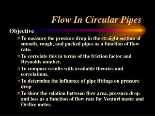
Flow In Circular Pipes. Objective To measure the pressure drop in the straight section of smooth, rough, and packed pipes as a function of flow rate. To correlate this in terms of the friction factor and Reynolds number. To compare results with available theories and correlations.

E N D
Flow In Circular Pipes Objective • To measure the pressure drop in the straight section of smooth, rough, and packed pipes as a function of flow rate. • To correlate this in terms of the friction factor and Reynolds number. • To compare results with available theories and correlations. • To determine the influence of pipe fittings on pressure drop • To show the relation between flow area, pressure drop and loss as a function of flow rate for Venturi meter and Orifice meter.
APPARATUS Pipe Network Rotameters Manometers
Theoretical Discussion • Fluid flow in pipes is of considerable importance in process. • Animals and Plants circulation systems. • In our homes. • City water. • Irrigation system. • Sewer water system • Fluid could be a single phase: liquid or gases • Mixtures of gases, liquids and solids • NonNewtonian fluids such as polymer melts, mayonnaise • Newtonian fluids like in your experiment (water)
Theoretical DiscussionLaminar flow To describe any of these flows, conservation of mass and conservation of momentum equations are the most general forms could be used to describe the dynamic system. Where the key issue is the relation between flow rate and pressure drop. • If the flow fluid is: • Newtonian • Isothermal • Incompressible (dose not depend on the pressure) • Steady flow (independent on time). • Laminar flow (the velocity has only one single component)
Laminar flow Navier-Stokes equations is govern the flow field (a set of equations containing only velocity components and pressure) and can be solved exactly to obtain the Hagen-Poiseuille relation . Pz Flow If the principle of conservation of momentum is applied to a fixed volume element through which fluid is flowing and on which forces are acting, then the forces must be balanced (Newton second law) Vz(r) Pz+dz In Body force due to gravity r+dr r Pz+dz
Laminar flowContinue Forces balance Pz 1…Shear forces Vz(r) Pz+dz 2….Pressure r+dr r 3…..Body force
Laminar flowContinue Momentum is Mass*velocity (m*v) Momentum per unit volume is *vz Rate of flow of momentum is *vz*dQ dQ=vz2πrdr but vz = constant at a fixed value of r Laminar flow
Laminar flowContinue Hagen-Poiseuille
uz Uz average úz ur Ur average úr p paverage P’ Time Turbulent flow • When fluid flow at higher flowrates, the streamlines are not steady and straight and the flow is not laminar. Generally, the flow field will vary in both space and time with fluctuations that comprise "turbulence • For this case almost all terms in the Navier-Stokes equations are important and there is no simple solution • P = P (D, , , L, U,)
Turbulent flow All previous parameters involved three fundamental dimensions, Mass, length, and time From these parameters, three dimensionless groups can be build
Friction Factor for Laminar Turbulent flows From forces balance and the definition of Friction Factor Ac: cross section area of the pip S: Perimeter on which T acts (wetted perimeter) Rh hydraulic radius For Laminar flow (Hagen - Poiseuill eq) For Turbulent Flow
Turbulence: Flow Instability • In turbulent flow (high Reynolds number) the force leading to stability (viscosity) is small relative to the force leading to instability (inertia). • Any disturbance in the flow results in large scale motions superimposed on the mean flow. • Some of the kinetic energy of the flow is transferred to these large scale motions (eddies). • Large scale instabilities gradually lose kinetic energy to smaller scale motions. • The kinetic energy of the smallest eddies is dissipated by viscous resistance and turned into heat. (=head loss)
Velocity Distributions • Turbulence causes transfer of momentum from center of pipe to fluid closer to the pipe wall. • Mixing of fluid (transfer of momentum) causes the central region of the pipe to have relatively constant velocity (compared to laminar flow) • Close to the pipe wall eddies are smaller (size proportional to distance to the boundary)
Surface Roughness Additional dimensionless group /D need to be characterize Thus more than one curve on friction factor-Reynolds number plot Fanning diagram or Moody diagram Depending on the laminar region. If, at the lowest Reynolds numbers, the laminar portion corresponds to f =16/Re Fanning Chart or f = 64/Re Moody chart
Smooth pipe, Re>3000 Rough pipe, [ (D/)/(Re√ƒ) <0.01] Transition function for both smooth and rough pipe Friction Factor for Smooth, Transition, and Rough Turbulent flow
Fanning Diagram f =16/Re
Must be dimensionless! Pipe roughness pipe material pipe roughness (mm) glass, drawn brass, copper 0.0015 commercial steel or wrought iron 0.045 asphalted cast iron 0.12 galvanized iron 0.15 cast iron 0.26 concrete 0.18-0.6 rivet steel 0.9-9.0 corrugated metal 45 0.12 PVC
Flow in a Packed pipe The equations for empty pipe flow do not work with out considerable modification Ergun Equation A Dp Dp is the particle diameter, is the volume fraction that is not occupied by particles Flow Reynolds number for a packed bed flow as This equation contains the interesting behavior that the pressure drop varies as the first power of Uo for small Re and as Uo2 for higher Re.
Energy Loss in Valves • Function of valve type and valve position • The complex flow path through valves can result in high head loss (of course, one of the purposes of a valve is to create head loss when it is not fully open) • Ev are the loss in terms of velocity heads
0.8 0.7 0.6 0.5 KE 0.4 0.3 0.2 0.1 0 0 20 40 60 80 Energy Loss due to Gradual Expansion A1 A2 angle ()
P1 P2 D d 1 0.95 0.9 0.85 Cd 0.8 0.75 0.7 0.65 0.6 102 105 106 107 Re Sudden Contraction (Orifice Flowmeter) Orifice flowmeters are used to determine a liquid or gas flowrate by measuring the differential pressure P1-P2 across the orifice plate Flow 103 104 Reynolds number based on orifice diameter Red
D Flow d Venturi Flowmeter The classical Venturi tube (also known as the Herschel Venturi tube) is used to determine flowrate through a pipe. Differential pressure is the pressure difference between the pressure measured at D and at d
v v Boundary layer buildup in a pipe Because of the share force near the pipe wall, a boundary layer forms on the inside surface and occupies a large portion of the flow area as the distance downstream from the pipe entrance increase. At some value of this distance the boundary layer fills the flow area. The velocity profile becomes independent of the axis in the direction of flow, and the flow is said to be fully developed. Pipe Entrance v
Pipe Flow Head Loss(constant density fluid flows) • Pipe flow head loss is • proportional to the length of the pipe • proportional to the square of the velocity (high Reynolds number) • Proportional inversely with the diameter of the pipe • increasing with surface roughness • independent of pressure • Total losses in the pipe system is obtained by summing individual head losses of roughness, fittings, valves ..itc
Pipe Flow Summary • The statement of conservation of mass, momentum and energy becomes the Bernoulli equation for steady state constant density of flows. • Dimensional analysis gives the relation between flow rate and pressure drop. • Laminar flow losses and velocity distributions can be derived based on momentum and mass conservation to obtain exact solution named of Hagen - Poisuille • Turbulent flow losses and velocity distributions require experimental results. • Experiments give the relationship between the fraction factor and the Reynolds number. • Head loss becomes minor when fluid flows at high flow rate (fraction factor is constant at high Reynolds numbers).
Images - Laminar/Turbulent Flows Laser - induced florescence image of an incompressible turbulent boundary layer Laminar flow (Blood Flow) Simulation of turbulent flow coming out of a tailpipe Turbulent flow Laminar flow http://www.engineering.uiowa.edu/~cfd/gallery/lim-turb.html
Pipes are Everywhere! Owner: City of Hammond, INProject: Water Main RelocationPipe Size: 54"