FLOW IN PIPES
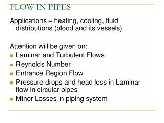
FLOW IN PIPES. Applications – heating, cooling, fluid distributions (blood and its vessels) Attention will be given on: Laminar and Turbulent Flows Reynolds Number Entrance Region Flow Pressure drops and head loss in Laminar flow in circular pipes Minor Losses in piping system.

FLOW IN PIPES
E N D
Presentation Transcript
FLOW IN PIPES Applications – heating, cooling, fluid distributions (blood and its vessels) Attention will be given on: • Laminar and Turbulent Flows • Reynolds Number • Entrance Region Flow • Pressure drops and head loss in Laminar flow in circular pipes • Minor Losses in piping system
Define and explain Laminar and turbulent flows in pipes, Reynolds number, and Critical Reynolds Number. • Explain friction loss in Laminar flow. Derive and Explain Hagen - Poiseuille equation. • Explain and describe the important of Poiseuille’s law in Biomedical application. • Explain the important of laminar and turbulent flow in biomedical engineering. • Solve problems about laminar and turbulent flow.
FLOW IN PIPES Fluid flow can be classified as external or internal. We focus on internal for flow in pipes.
LAMINAR AND TURBULENT FLOWS The flow appears to be smooth and steady. The stream has a fairly uniform diameter and there is little or no evidence of mixing of the various parts of the stream. The flow has very low velocity – highly ordered motion The flow has a rather high velocity – highly disordered motion. The elements of fluid appear to be mixing chaotically within the stream.
REYNOLDS NUMBER How to distinguish Turbulent and Laminar in mathematics? Osborne Reynolds manage to do that in 1880s. Re = vDρ/µ where fluid density ρ, fluid viscosity µ, pipe diameter D, and average velocity of flow, v. Re is the ratio of the inertial forces to viscous forces in the fluid. Dimensionless - no UNITS. How to calculate average velocity,v in laminar flow? The mean velocity is half of the maximum velocity. Vmean = Vmax/2
REYNOLDS NUMBER How to use it ? Critical Reynolds Number – flow become turbulent. Larger Re – Inertial is bigger than viscous, viscous cannot prevent the random and rapid fluctuation of the fluids and vice versa. The Re value is different for different geometries and flow conditions. For circular pipe, Recr = 2300.
EXAMPLE 1–REYNOLDS NUMBER Determine whether the flow is laminar or turbulent if glycerine at 25°C flows in a pipe with a 150-mm inside diameter. The average velocity of flow is 3.6 m/s. We must first evaluate the Reynolds number
Laminar and Turbulent in Human Blood Most of human blood flow is laminar, having Re of 300 or less. However, it is possible for turbulent to occur at very high flow rates in the descending aorta, for example in highly conditioned athletes. Sometimes it is also common in pathological conditions (narrowed (stenotic) arteries and across stenotic heart valves.
TURBULENT AND ITS EFFECT • Haemodynamic studies have shown that diseased cardiac valves, whether stenosed or incompetent, create regions of increased turbulence and shear stresses that are large enough to damage the vascular endothelium leading to endothelial dysfunction. • Endothelial cells line the entire circulatory system, from the heart to the smallest capillary. These cells reduce friction of the flow of blood allowing the fluid to be pumped further and control of blood pressure. • A key feature of endothelial dysfunction is the inability of arteries and arterioles to dilate fully in response to an appropriate stimulis.
Laminar and Turbulent in the lungs In the lungs, fully developed laminar flow probably occurs only in very small airways with low Re. When air flow at higher rates in larger diameter tubes, like Trachea, the flow is often turbulent. Much of the flow in intermediate sized airways will be transitional flow.
ENTRANCE REGIONFLOW ENTERING CIRCULAR PIPE Boundary layer region - Viscous effects and the velocity changes are significance The inviscid flow region – Frictional effects are negligible and velocity in radial directions is constant. The region from the pipe inlet to the point at which the boundary layer merges at the centreline is called the Hydrodynamic Entrance Region, and the length is Hydrodynamic Entry Length, Lh.
ENTRY LENGTH (LENGTH OF ENTRANCE REGION), Lh Laminar flow, Turbulent flow, For a pipe length over than 10D, entrance effect is negligible and thus,
FULLY DEVELOP FLOW IN ARTERIES If we consider Re = 300, then the previous equation gives Xe=18D. This means that, an entrance length equal to 18 pipe diameters is required for fully developed flow in human system. In human cardiovascular system, it is not common to see fully developed flow in arteries. The vessels continually branch, with the distance between branches not often being greater than 18 diameters.
LAMINAR FLOW IN PIPES • Assumptions: • Steady, laminar flow of incompressible liquid with constant properties in the fully developed region of a straight circular pipe • No acceleration since it is steady and fully develop. • No motion in the radial direction, velocity in radial direction is zero • We try to obtain the velocity profile and also a relation to the friction factor.
LAMINAR FLOW IN PIPES • Consider a free-body diagram of the cylinder of fluid and sum the forces acting on that cylinder. • First, we will need to make some assumptions. Assume that the flow is steady. This means that the flow is not changing with time; that the derivative of flow rate with respect to time is equal to zero.
LAMINAR FLOW IN PIPES • Second, assume that the flow is through a long tube with a constant cross-section. This flow condition is known as uniform flow. For steady flows in long tubes with a constant cross-section, the flow is fully developed and therefore, the pressure gradient, dP/dx is constant.
LAMINAR FLOW IN PIPES • The third assumption is that the fluid is Newtonian. Newtonian flow is flow in which the shearing stress, t, in the fluid is constant. In other words, the viscosity is constant with respect to the shear rate, y, and the whole process is carried out at a constant temperature.
LAMINAR FLOW IN PIPES • Now let the x direction be the axial direction of the pipe with the downstream (to the right) being positive.If the flow is unchanging with time, then the sum of forces in the x dire< P(πr2) - (P + dP)(πr2) – τ2πrdx = 0 • Solve Eq. (1.1) and the result is -dP(πr2) = 2πrτdx
LAMINAR FLOW IN PIPES • The result from a simple force balance is shear stress as a function of pressure gradient, dP/dx and radial position, r: and
LAMINAR FLOW IN PIPE • From the definition of viscosity that the shear stress is also related to the shear rate: From the relation of shear stress, pressure drop and velocity gradient Then producing differential equation with the variables velocity,V and radius,r:
LAMINAR FLOW IN PIPE • The next step in the analysis is to solve the previous differential equation, which gives the velocity of each point in the tube as a functionof the radius, r:
LAMINAR FLOW IN PIPE • So far, in this analysis, we have made three assumptions. First, steady flow (dQ/dt = 0); second, fully developed tube (dP/dx is constant); and third, viscosity is constant. • Now we make assumption four, which is the no slip condition. This means V at the wall is zero when r equals the radius of the tube. Therefore, set r = Rtube = R and V=0 to solve for C1.
LAMINAR FLOW IN PIPE The equation, which gives velocity as a function of radius, r, is then The final assumption is that the flow is laminar whereby this parabolic velocity profile represents the velocity profile across a constant cross section.
LAMINAR FLOW IN PIPES; VELOCITY PROFILE The dP/dx must have –ve value for pressure drops that cause a positive velocity (pressure must decrease in the flow direction due to the viscous effect). The maximum velocity will occur at the centreline, where r=0. In fluid flow, it is convenient to work with average velocity which remains constant in incompressible flow when the cross sectional area of pipe is constant.
PRESSURE DROP Pressure drop occurs as the fluid flows along straight lengths of pipe and tubing. It causes pressure to decrease along the pipe and they increase the amount of power that a pump must deliver the fluid. It is caused by friction, changes in kinetic energy, etc. Friction may occur between the fluid & the pipe work, but friction also occurs within the fluid as sliding between adjacent layers of fluid takes place. The friction within the fluid is due to the fluid’s viscosity. When fluids have a high viscosity, the speed of flow tends to be low, and resistance to flow becomes almost totally dependant on the viscosity of the fluid, this condition is known as ‘Laminar flow’.
PRESSURE DROP IN LAMINAR FLOW In laminar flow, the fluid seems to flow in several layers, one on another as described in below figures. Because of the viscosity, shear stress is created between the layers of fluid. WHY ENERGY IS LOST ??? Overcoming the frictional forces produced by the shear stress (act opposite direction to flow).
PRESSURE DROP IN LAMINAR FLOW The pressure drop in laminar flow can be expressed as below. Pressure drop will be 0 if the viscosity is 0, when there is no frictions. It also mean that the pressure drop depends entirely on the viscous effects.
PRESSURE DROP The above equation is used to determine the pressure drop in laminar flow. However, the following equation can be used to determine the pressure drop for all cases of fully develop internal flow (Laminar or Turbulent, Circular or non circular pipes, Smooth or rough surfaces, Horizontal or inclines) and known as Darcy’s equation. Where friction factors, f can be defined as
PRESSURE DROP IN LAMINAR Both (1) and (2) equation can be used to determine the pressure drop for circular pipe in laminar flow, equating both, we find, The equation shows that for laminar flow the friction factors is a function of Reynolds number only and independent of surface roughness.
HEAD LOSS In piping system analysis, ΔP =ρgh express loss in terms of pressure. The pressure loss can also be expressed in terms of length of water (m) which is hL=ΔPL/pg It represents the additional height that the fluid need to be raised by a pump to overcome the frictional losses in the pipe.
R X MEAN VELOCITY AND FLOW RATE • Consider the steady,laminar flow in pipe as shown in the above figure. • The velocity of the fluid is the function of radius,r and distance x and can be shown as u(r,x). • Since dQ/dt=0, conservation of mass equation is applied, mass flow rate,dm/dt and mean velocity,Vm relation can be define as
MEAN VELOCITY AND FLOW RATE Then Vm can be expressed as For fully developed flow in pipe, the velocity is constant through the flow direction, therefore,
MEAN VELOCITY AND FLOW RATE Thus velocity can be expressed as From (a) and (b), the mean velocity then can be expressed as From (c) and (d), the relation between mean velocity and velocity at any radius, Mean velocity, Vm is at radius r=0, therefore
MEAN VELOCITY AND FLOW RATE Combining the relation between Pressure Drop and Mean velocity in laminar flow, we obtained the following relationship. The flow rate is This relationship is known as the Hagen–Poiseuille equation. The equation is valid only for laminar flow (NR< 2000).
EXAMPLE 2 - ENERGY LOSS Determine the energy loss if glycerine at 25°C flows 30 m through a 150-mm-diameter pipe with an average velocity of 4.0 m/s. First, we must determine whether the flow is laminar or turbulent by evaluating the Reynolds number: From Appendix B, we find that for glycerin at 25°C
EXAMPLE 2 - ENERGY LOSS Because NR< 2000, the flow is laminar. Using Darcy’s equation, we get Notice that each term in each equation is expressed in the units of the SI unit system. Therefore, the resulting units for hL are m or Nm/N. This means that 13.2 Nm of energy is lost by each newton of the glycerine as it flows along the 30 m of pipe.
POISEUILLE’S LAW AND AIR RESISTANCE IN PULMONARY When we breathe air flows through trachea to the lungs. Although the air is not very viscous, there is a noticeable resistance to the air flow. It causes the pressure drop along the airway and it decrease in the direction of the flow. When air flows through relatively small diameters tubes as in the terminal brochioles, the flow is laminar. When it flows at higher rates in larger diameter tubes, like the trachea, the flow is often turbulent. Much of the flow in the intermediate sized airways can be transitional flow which is difficult to predict either laminar or turbulent.
POISEUILLE’S LAW AND AIR RESISTANCE IN PULMONARY We learn about Poiseuille’s law that relevant to laminar flow. This law applies to air flow and also blood flow. The relation can be expressed as below Analogous to V=IR in electrical, Voltage drop,V similar to Pressure gradient, ΔP/L; electric current similar to flow rate and resistance to flow can be expressed as Resistance is inversely related to the fourth power of the diameter, the resistance in the airways is not predominantly in the smallest diameter airways. Why? See next slide.
POISEUILLE’S LAW AND AIR RESISTANCE IN PULMONARY Airways branches and become narrower, but they are also numerous. Therefore the smaller bronchioles contribute relatively little resistance because of their increased numbers. The major site of airway resistance is the medium-sized bronchi. Airways with less than 2mm diameter only contribute about 20% of air resistance. 25 -40% is contributed by upper airways including the mouth, nose, pharynx, larynx and trachea.
FRICTION LOSS IN TURBULENT FLOW • Using Darcy equations we can calculate the friction losses in turbulent flow. It depends on the surface roughness of the pipe as well as Reynolds number (IN LAMINAR, LOSSES ONLY DEPEND ON THE REYNOLD NUMBER) • The є , the average wall roughness can be obtained from tables (experiment has been conducted to determine the value). The average value is for new and clean pipe.
FRICTION LOSS IN TURBULENT FLOW Roughness value, є for new and clean pipe
MOODY DIAGRAM FOR TURBULENT FLOW • One of the most widely used methods for evaluating the friction factor employs the Moody diagram shown below.
MOODY DIAGRAM –IMPORTANT OBSERVATION For a given Reynolds number of flow, as the relative roughness is increased, the friction factor f decreases. For a given relative roughness , the friction factor f decreases with increasing Reynolds number until the zone of complete turbulence is reached.
MOODY DIAGRAM The transition region is shown in the shaded area (2300<Re<4000) The friction factors alternate between laminar and turbulent flow.
MOODY DIAGRAM Within the zone of complete turbulence, the Reynolds number has no effect on the friction factor. As the relative roughness increases, the value of the Reynolds number at which the zone of complete turbulence begins also increases. The friction factor is a minimum for a smooth pipe (but still not zero because of the no-slip condition) and increases with roughness.
READING THE MOODY DIAGRAM • Check your ability to read the Moody diagram correctly by verifying the following values for friction factors for the given values of Reynolds number and relative roughness, using Fig. 8.6:
USE OF THE MOODY DIAGRAM Why do we need the Moody diagram? The Moody diagram is used to help determine the value of the friction factor, ffor turbulent flow. How ? • First determine the value of the Reynolds number (calculations), • Then determine the relative roughness (dividing Diameter of the pipe to the pipe roughness). Therefore, the basic data required are: 1. The pipe inside diameter, 2. The pipe material, 3. The flow velocity, and the kind of fluid and its temperature, from which the viscosity can be found.
EXAMPLE 3- MOODY DIAGRAM Determine the friction factor f if water at 70°C is flowing at 9.14 m/s in an uncoated ductile iron pipe having an inside diameter of 25 mm. The Reynolds number must first be evaluated to determine whether the flow is laminar or turbulent: Here D=0.025 m and kinematic viscosity=4.11x10⁻⁷ m2/s. We now have
EXAMPLE 3- MOODY DIAGRAM Thus, the flow is turbulent. Now the relative roughness must be evaluated. From Table 8.2 we find ε= 2.4 x 10⁻⁴ m. Then, the relative roughness is The steps are as follows: 1. Locate the Reynolds number on the abscissa of the Moody diagram:
EXAMPLE 3- MOODY DIAGRAM 2. Project vertically until the curve for D/ε = 104 is reached. Because 104 is so close to 100, that curve can be used. 3. Project horizontally to the left, and read f = 0.038.