Computer-Aided Molecular Modeling of Materials

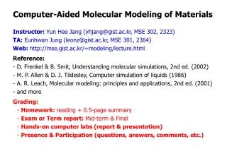
1. Computer-Aided Molecular Modeling of Materials Instructor: Yun Hee Jang (yhjang@gist.ac.kr, MSE 302, 2323) TA: Eunhwan Jung (leonz@gist.ac.kr, MSE 301, 2364) Web: http://mse.gist.ac.kr/~modeling/lecture.html Reference: - D. Frenkel & B. Smit, Understanding molecular simulations, 2nd ed. (2002) - M. P. Allen & D. J. Tildesley, Computer simulation of liquids (1986) - A. R. Leach, Molecular modeling: principles and applications, 2nd ed. (2001) - and more Grading: - Homework: reading + 0.5-page summary - Exam or Term report: Mid-term & Final - Hands-on computer labs (report & presentation) - Presence & Participation (questions, answers, comments, etc.)

2. Why do we need a molecular modeling (i.e. computer simulation at a molecular level) in materials science? Emerging (future) Materials science N~102, L~10 nm Simulation will lead. Traditional (Past) Materials science N~1023, L~10 cm Experiment didn’t need simulation. Molecular simulation in virtual space Difficulty (cost, time, manpower, inaccuracy) too hard hard Experiment in real space easy easy N(number of atoms) or L (size) of a system of interest)

3. Nobel Prize History of Molecular Modeling • 1918 – Physics – Max Planck – Quantum theory of blackbody radiation • 1921 – Physics – Albert Einstein– Quantum theory of photoelectric effect • 1922 – Physics – Niels Bohr – Quantum theory of hydrogen spectra • 1929 – Physics – Louis de Broglie – Matter waves • 1932 – Physics – Werner Heisenberg – Uncertainty principle • 1933 – Physics – Erwin Schrodinger & Paul Dirac – Wave equation • 1945 – Physics – Wolfgang Pauli – Exclusion principle • 1954 – Physics – Max Born – Interpretation of wave function • 1998 – Chemisty – Walter Kohn & John Pople • 2013 – Chemisty – Martin Karplus, Michael Levitt, Arieh Warshel Quantum Mechanics Quantum Chemistry Classical Molecular Simulation

4. Review of Nobel Information 2013 Chemistry • Simulation or Modeling of molecules (in materials) on computers • Classical (Newtonian) physics vs. Quantum (Schrodinger) physics • Quantum description of atoms and molecules: electrons & nuclei • Strength: applicable to describe electronic (photo)excitation • Strength: interatomic interactions described “naturally” • Strength: chemical reactions (bond formation/breaking) • Weakness: slow, expensive, small-scale (N < 102), @ 0 K • Classical description of atoms and molecules: balls & springs • Strength: fast, applicable to large-scale (large N) systems • Strength: close to our conventional picture of molecules • Strength: easy to code, free codes available, finite T • Weakness: interatomic interactions from us (force field) • Weakness: no chemical reactions, no electronic excitation • Application: structural, mechanical, dynamic properties

5. Quantum vs. Classical description of materials With reasonable amount of resources, larger-scale (larger-N) systems can be described with classical simulations than with quantum simulations. Quantum simulation in virtual space Difficulty (cost, time, manpower, inaccuracy) Classical simulation in virtual space hard Experiment in real space easy N(number of atoms) or L (size) of a system of interest)

6. Example of multi-scale molecular modeling: CO2 capture project MC Monte Carlo Process Simulation - Grand Canonical (GCMC) or Kinetic (KMC) - Flue gas diffusion & Selective CO2 capture MD Large-scale Molecular Dynamics - Validation: Interatomic potential (Force Field) - Viscosity, diffusivity distribution: bulk solvent QM First-principles Quantum Mechanics - Validation: DFT + continuum solvation - Reaction: solvent molecule + CO2 complex

7. PzH3+-CO2 Step 1: Quantum: Reaction N H 10.6 kcal/mol (MEA) +CO2 PzH+-2CO2- C Piperazine O 7.8 PzH2+-CO2- +PzH2 +PzH2 +CO2 PzH-CO2H PzH3+ Pz(CO2)22- +CO2 PzH3+ PzHCO2- solvent (PzH2) PzH2 (regener) PzH2+CO2- PzH3+ HCO3-

8. Quantum simulation Example No. 2: Pd촉매 반응, UV/vis spectrum 재현,유기태양전지 효율 저하 설명 - 1.96 PCE 3.1% - 3.26 EX2 EX1 3.26 1.96 - 5.22 - 2.12 PCE 0.4% EX1 gone! 2.99 - 5.11 8.9 0 -18.4 -26.5 -29.1 -32.4 -34.7 -51.3 Pd+ 22BI Pd++2BI TS1 I3 I1 TS2 I2 TS3

9. What quantum/classical molecular modeling can bring to you: Examples. Reduction-oxidation potential, acibity/basicity (pKa), UV-vis spectrum, density profile, etc. J. Phys. Chem. B (2006) J. Phys. Chem. A (2009, 2001), J. Phys. Chem. B (2003), Chem. Res. Toxicol. (2003, 2002, 2000), Chem. Lett. (2007) J. Phys. Chem. B (2011), J. Am. Chem. Soc. (2005, 2005, 2005) cm-1

10. Step 2: Classical: 2-species (AMP and PZ) distribution in water Which one (among AMP and PZ) is less soluble in water? Which one is preferentially positioned at the gas-liquid interface? Which one will meet gaseous CO2 first? Hopefully PZ to capture CO2 faster, but is it really like that? Let’s see with the MD simulation on a model of their mixture solution!

11. First-principles multi-scale molecular modeling • 제일원리 다단계 분자모델링 • ► 물질구조 분자수준 이해► 선험적 특성 예측 • ► 신물질 설계 ►물질특성 향상 2. 고전역학 분자동력학 모사 (컴퓨터 구축 102~107개 원자계의 뉴턴방정식 풀기) - 전자 무시, ball (원자) & spring (결합) 모델로 분자/물질 표현 (힘장) - Cheap ► 대규모 시스템에 적용, 시간/온도에 따른 구조/형상 변화 모사 1. 양자역학 전자구조 계산 (컴퓨터 구축 101~103개 원자계 슈레딩거방정식 풀기) - 정확, 경험적 패러미터 불필요, 제일원리계산, but expensive ► 소규모 시스템 snapshot CG-FF MD atomistic molecular CGMD coarse- grained understanding new design prediction EXPERIMENT synthesis fabrication characterization MULTI SCALE MODELING nanoscale morphology FF test validation QM electronic structure KMC charge- transport transport parameter

12. Lecture series I-IV: Molecular Modeling of Materials • I. 2013 Spring: Elements of Quantum Mechanics (QM) • - Birth of quantum mechanics, its postulates & simple examples • Particle in a box (translation) • Harmonic oscillator (vibration) • Particle on a ring or a sphere (rotation) • II. 2013 Fall: Quantum Chemistry • - Quantum-mechanical description of chemical systems • One-electron & many-electron atoms • Di-atomic & poly-atomic molecules • III. 2014 Spring: Classical Molecular Simulations of materials • - Large-scale simulation of chemical systems (or any collection of particles) • Monte Carlo (MC) & Molecular Dynamics (MD) • IV. 2014 Fall: Molecular Modeling of Materials (Project-oriented class) • - Application of a combination of the above methods to understand • structures, electronic structures, properties, and functions of various materials

13. A typical experiment in a real (not virtual) space • Some material is put in a container at fixed T & P. • The material is in a thermal fluctuation, producing lots of different configurations (a set of microscopic states) for a given amount of time. It is the Mother Nature who generates all the microstates. • An apparatus is plugged to measure an observable (a macroscopic quantity) as an average over all the microstates produced from thermal fluctuation. P P T T How do we mimic the Mother Nature in a virtual space to realize lots of microstates, all of which correspond to a given macroscopic state? How do we mimic the apparatus in a virtual space to obtain a macroscopic quantity (or property or observable) as an average over all the microstates? P T

14. How do we mimic the Mother Nature in a virtual space to realize lots of microstates, all of which correspond to a given macroscopic state? By MC & MD methods! microscopic states (microstates) or microscopic configurations under external constraints (N or , V or P, T or E, etc.)  Ensemble (micro-canonical, canonical, grand canonical, etc.) In a real-space experiment In a virtual-space simulation Average over a collection of microstates they’re generated naturally from thermal fluctuation it is us who needs to generate them by QM/MC/MD methods. Macroscopic quantities (properties, observables) These are what are measured in true experiments. • thermodynamic –  or N, E or T, P or V, Cv, Cp, H, S, G, etc. • structural – pair correlation function g(r), etc. • dynamical – diffusion, etc.