Microarray Data Normalization and Error Models: Methods and Applications
This presentation by Wolfgang Huber from EMBL-EBI, delivered in Brixen on June 16, 2008, focuses on the intricacies of microarray data normalization. It discusses various error models affecting the quality of oligonucleotide microarrays, the importance of normalization to mitigate biases, and the statistical methods necessary to ensure data accuracy. With insights into probe sets, mismatches, and the impacts of RNA extraction and labeling efficiencies, this session is invaluable for researchers aiming to enhance the reliability of their microarray analyses.

Microarray Data Normalization and Error Models: Methods and Applications
E N D
Presentation Transcript
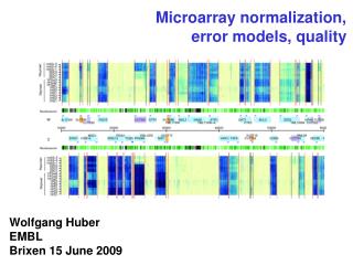
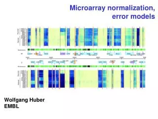
Microarray normalization, error models, quality Wolfgang Huber EMBL-EBI Brixen 16 June 2008
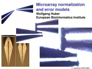
* * * * * Oligonucleotide microarrays GeneChip Hybridized Probe Cell Target - single stranded cDNA Oligonucleotide probe 5µm Millions of copies of a specific oligonucleotide probe molecule per patch 1.28cm up to 6.5 Mio different probe patches Image of array after hybridisation and staining
Each target molecule (transcript) is represented by several oligonucleotides of (intended) length 25 bases Probe: one of these 25-mer oligonucleotides Perfect match (PM): A probe exactly complementary to the target sequence Mismatch (MM): same as PM but with a single homomeric base change for the middle (13th) base (G-C, A-T) Probe-pair: a (PM, MM) pair. Probe set: a collection of probe-pairs (e.g. 11) targeting the same transcript MGED/MIAME: „probe“ is ambiguous! Reporter: the sequence Feature: a physical patch on the array with molecules intended to have the same reporter sequence (one reporter can be represented by multiple features) Terminology for transcription arrays
Image analysis • about 100 pixels per feature • segmentation • summarisation into one number representing the intensity level for this feature • CEL file
samples: mRNA from tissue biopsies, cell lines fluorescent detection of the amount of sample-probe binding arrays: probes = gene-specific DNA strands tissue A tissue B tissue C ErbB2 0.02 1.12 2.12 VIM 1.1 5.8 1.8 ALDH4 2.2 0.6 1.0 CASP4 0.01 0.72 0.12 LAMA4 1.32 1.67 0.67 MCAM 4.2 2.93 3.31 marray data
bias From: lymphoma dataset vsn package Alizadeh et al., Nature 2000
MA-plot M A
log2 intensity arrays / dyes
Non-linearity log2 Cope et al. Bioinformatics 2003
ratio compression nominal 3:1 nominal 1:1 nominal 1:3 Yue et al., (Incyte Genomics) NAR (2001) 29 e41
A complex measurement process lies between mRNA concentrations and intensities The problem is less that these steps are ‘not perfect’; it is that they vary from array to array, experiment to experiment.
tumor-normal log-ratio Which genes are differentially transcribed? same-same
Statistics 101: biasaccuracy precision variance
Basic dogma of data analysis Can always increase sensitivity on the cost of specificity, or vice versa, the art is to - optimize both, then - find the best trade-off. X X X X X X X X X
How to compare microarray intensities with each other? How to address measurement uncertainty (“variance”)? How to calibrate (“normalize”) for biases between samples? Questions
Systematic Stochastic o similar effect on many measurements o corrections can be estimated from data o too random to be ex-plicitely accounted for o remain as “noise” Calibration Error model Sources of variation amount of RNA in the biopsy efficiencies of -RNA extraction -reverse transcription -labeling -fluorescent detection probe purity and length distribution spotting efficiency, spot size cross-/unspecific hybridization stray signal
Ben Bolstad 2001 Quantile normalisation
data("Dilution") nq = normalize.quantiles(exprs(Dilution)) nr = apply(exprs(Dilution), 2, rank) for(i in 1:4) plot(nr[,i], nq[,i], pch=".", log="y", xlab="rank", ylab="quantile normalized", main=sampleNames(Dilution)[i])
Quantile normalisation is: per array rank-transformation followed by replacing ranks with values from a common reference distribution
+ Simple, fast, easy to implement + Always works, needs no user interaction / tuning + Non-parametric: can correct for quite nasty non-linearities (saturation, background) in the data - Always "works", even if data are bad / inappropriate - Conservative: rank transformation looses information - may yield less power to detect differentially expressed genes - Aggressive: when there is an excess of up- (or down) regulated genes, it removes not just technical, but also biological variation Quantile normalisation
loess (locally weighted scatterplot smoothing): an algorithm for robust local polynomial regression by W. S. Cleveland and colleagues (AT&T, 1980s) and handily available in R "loess" normalisation
Local polynomial regression bandwidth b
C. Loader Local Regression and Likelihood Springer Verlag
loess normalisation • local polynomial regression of M against A • 'normalised' M-values are the residuals before after
n-dimensional local regression model for microarray normalisation An algorithm for fitting this robustly is described (roughly) in the paper. They only provided software as a compiled binary for Windows. The method has not found much use.
3000 3000 x3 ? 1500 200 1000 0 ? x1.5 A A B B C C But what if the gene is “off” (below detection limit) in one condition? ratios and fold changes Fold changes are useful to describe continuous changes in expression
ratios and fold changes The idea of the log-ratio (base 2) 0: no change +1: up by factor of 21 = 2 +2: up by factor of 22 = 4 -1: down by factor of 2-1 = 1/2 -2: down by factor of 2-2 = ¼ A unit for measuring changes in expression: assumes that a change from 1000 to 2000 units has a similar biological meaning to one from 5000 to 10000. What about a change from 0 to 500? - conceptually - noise, measurement precision
Many data are measured in definite units: time in seconds lengths in meters energy in Joule, etc. Climb Mount Plose (2465 m) from Brixen (559 m) with weight of 78 kg, working against a gravitation field of strength 9.81 m/s2 : What is wrong with microarray data? (2465 - 559) · 78 · 9.81 m kg m/s2 = 1 458 433 kg m2 s-2 = 1 458.433 kJ
Robust affine regression normalisation (n-dim.) with the additive-multiplicative error model Error model: Trey Ideker et al. (2000) JCB David Rocke and Blythe Durbin: (2001) JCB, (2002) Bioinformatics Use for robust affine regression normalisation: W. Huber, Anja von Heydebreck et al. (2002) Bioinformatics
bi per-sample gain factor bk sequence-wise probe efficiency hik multiplicative noise ai per-sample offset eik additive noise The two component model measured intensity = offset + gain true abundance
“multiplicative” noise “additive” noise The two-component model raw scale log scale B. Durbin, D. Rocke, JCB 2001
Parameterization two practically equivalent forms (h<<1)
variance stabilizing transformations Xu a family of random variables with E Xu = u, Var Xu = v(u). Define Var f(Xu ) independent of u derivation: linear approximation
1.) constant variance (‘additive’) 2.) constant CV (‘multiplicative’) 3.) offset 4.) additive and multiplicative variance stabilizing transformations
the “glog” transformation - - - f(x) = log(x) ———hs(x) = asinh(x/s) P. Munson, 2001 D. Rocke & B. Durbin, ISMB 2002 W. Huber et al., ISMB 2002
generalized log-ratio difference log-ratio variance: constant part proportional part glog raw scale log glog