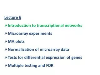
Lecture 9 Microarray experiments MA plots Normalization of microarray data
Lecture 9 Microarray experiments MA plots Normalization of microarray data Tests for differential expression of genes Multiple testing and FDR. DNA Microarray . Typical microarray chip. Though most cells in an organism contain the same genes, not all of the genes are used in each cell.

Lecture 9 Microarray experiments MA plots Normalization of microarray data
E N D
Presentation Transcript
Lecture 9 • Microarray experiments • MA plots • Normalization of microarray data • Tests for differential expression of genes • Multiple testing and FDR
DNA Microarray Typical microarray chip • Though most cells in an organism contain the same genes, not all of the genes are used in each cell. • Some genes are turned on, or "expressed" when needed in particular types of cells. • Microarray technology allows us to look at many genes at once and determine which are expressed in a particular cell type.
DNA Microarray Typical microarray chip • DNA molecules representing many genes are placed in discrete spots on a microscope slide which are called probes. • Messenger RNA--the working copies of genes within cells is purified from cells of a particular type. • The RNA molecules are then "labeled" by attaching a fluorescent dye that allows us to see them under a microscope, and added to the DNA dots on the microarray. • Due to a phenomenon termed base-pairing, RNA will stick to the probe corresponding to the gene it came from
DNA Microarray Usually a gene is interrogated by 11 to 20 probes and usually each probe is a 25-mer sequence The probes are typically spaced widely along the sequence Sometimes probes are choosen closer to the 3’ end of the sequence A probe that is exactly complementary to the sequence is called perfect match (PM) A mismatch probe (MM) is not complementary only at the central position In theory MM probes can be used to quantify and remove non specific hybridization Source: PhD thesis by Benjamin Milo Bolstad, 2004, University of California, Barkeley
Sample preparation and hybridization Source: PhD thesis by Benjamin Milo Bolstad, 2004, University of California, Barkeley
Sample preparation and hybridization During the hybridization process cRNA binds to the array Earlier probes had all the probes of a probset located continuously on the array This may fall prey to spatial defects Newer chips have all the probes spread out across the array A PM and MM probe pair are always adjacent on the array Source: PhD thesis by Benjamin Milo Bolstad, 2004, University of California, Barkeley
Growth curve of bacteria • Samples can be taken at different stages of the growth curve • One of them is considered as control and others are considered as targets • Samples can be taken before and after application of drugs • Sample can be taken under different experimental conditions e.g. starvation of some metabolite or so • What types of samples should be used depends on the target of the experiment at hand.
DNA Microarray Typical microarray chip • After washing away all of the unstuck RNA, the microarray can be observed under a microscope and it can be determined which RNA remains stuck to the DNA spots • Microarray technology can be used to learn which genes are expressed differently in a target sample compared to a control sample (e.g diseased versus healthy tissues) • However background correction and normalization are necessary before making useful decisions or conclusions
MA plots MA plots are typically used to compare two color channels, two arrays or two groups of arrays The vertical axis is the difference between the logarithm of the signals(the log ratio) and the horizontal axis is the average of the logarithms of the signals The M stands for minus and A stands for add MA is also mnemonic for microarray Mi= log(Xij) - log(Xik) = Log(Xij/Xik) (Log ratio) Ai=[log(Xij) + log(Xik)]/2 (Average log intensity)
A typical MA plot From the first plot we can see differences between two arrays but the non linear trend is not apparent This is because there are many points at low intensities compared to at high intensities MA plot allows us to assess the behavior across all intensities
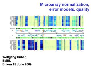
Normalization of microarray data Normalization is the process of removing unwanted non-biological variation that might exist between chips in microarray experiments By normalization we want to remove the non-biological variation and thus make the biological variations more apparent.
Normalization within individual arrays Sij = Xij- Xj Scaling: Cij= ( Xij- Xj ) / σj Centering:
Effect of Scaling and centering normalization Original Data Centering Scaling Mean = 0 Standard deviation = 1 Mean = 0
Normalization between a pair of arrays: Loess(Lowess) Normalization Lowess normalization is separately applied to each experiment with two dyes This method can be used to normalize Cy5 and Cy3 channel intensities (usually one of them is control and the other is the target) using MA plots
Normalization between a pair of arrays: Loess(Lowess) Normalization 2 channel data Mi=Log(Ti/Ci) (Log ratio) Ai=[log(Ti) + log(Ci)]/2 (Average log intensity) Mi=Log(Ti/Ci) Each point corresponds to a single gene Ai=[log(Ti) + log(Ci)]/2
Typical regression line Normalization between a pair of arrays: Loess(Lowess) Normalization Mi=Log(Ti/Ci) (Log ratio) Ai=[log(Ti) + log(Ci)]/2 (Average log intensity) Each point corresponds to a single gene Mi=Log(Ti/Ci) The MA plot shows some bias Ai=[log(Ti) + log(Ci)]/2
Normalization between a pair of arrays: Loess(Lowess) Normalization Mi=Log(Ti/Ci) (Log ratio) Ai=[log(Ti) + log(Ci)]/2 (Average log intensity) Each point corresponds to a single gene Mi=Log(Ti/Ci) The MA plot shows some bias Usually several regression lines/polynomials are considered for different sections Ai=[log(Ti) + log(Ci)]/2 The final result is a smooth curve providing a model for the data. This model is then used to remove the bias of the data points
Normalization between a pair of arrays: Loess(Lowess) Normalization Bias reduction by lowess normalization
Normalization between a pair of arrays: Loess(Lowess) Normalization Unnormalized fold changes fold changes after Loess normalization
Normalization across arrays Here we are discussing the following two normalization procedure applicable to a number of arrays • Quantile normalization • Baseline scaling normalization
Normalization across arrays Quantile normalization The goal of quantile normalization is to give the same empirical distribution to the intensities of each array If two data sets have the same distribution then their quantile- quantile plot will have straight diagonal line with slope 1 and intercept 0. Or projecting the data points of the quantile- quantile plot to 45-degree line gives the transformation to have the same distribution. quantile- quantile plot motivates the quantile normalization algorithm
Normalization across arrays Quantile normalization Algorithm Source: PhD thesis by Benjamin Milo Bolstad, 2004, University of California, Barkeley
Normalization across arrays QuantileNormalization: Original data Sort 1. Sort each column of X (values) 2. Take the means across rows of X sort Sort 3. Assign this mean to each element in the row to get X' sort 4. Get X normalized by rearranging each column of X' sort to have the same ordering as original X
Normalization across arrays Raw data After quantile normalization
Normalization across arrays Baseline scaling method In this method a baseline array is chosen and all the arrays are scaled to have the same mean intensity as this chosen array This is equivalent to selecting a baseline array and then fitting a linear regression line without intercept between the chosen array and every other array
Normalization across arrays Baseline scaling method
Normalization across arrays Raw data After Baseline scaling normalization
Tests for differential expression of genes Let x1…..xn and y1…yn be the independent measurements of the same probe/gene across two conditions. Whether the gene is differentially expressed between two conditions can be determined using statistical tests.
Tests for differential expression of genes • Important issues of a test procedure are • Whether the distributional assumptions are valid • Whether the replicates are independent of each other • Whether the number of replicates are sufficient • Whether outliers are removed from the sample • Replicates from different experiments should not be mixed since they have different characteristics and cannot be treated as independent replicates
Tests for differential expression of genes Most commonly used statistical tests are as follows: (a) Student’s t-test (b) Welch’s test (c) Wilcoxon’s rank sum test (d) Permutation tests The first two test assumes that the samples are taken from Gaussian distributed data and the p-values are calculated by a probability distribution function The later two are nonparametric and the p values are calculated using combinatorial arguments.
Student’s t-test Assumptions: Both samples are taken from Gaussian distribution that have equal variances Degree of freedom: m+n-2 Welch’s test is a variant of t-test where t is calculated as follows Welch’s test does not assume equal population variances
Student’s t-test The value of t is supposed to follow a t-distribution. After calculating the value of t we can determine the p-value from the t distribution of the corresponding degree of freedom
Wilcoxon’s rank sum test Let x1…..xn and y1…ym be the independent measurements of the same probe/gene across two conditions. Consider the combined set x1…..xn ,y1…ym The test statistic of Wilcoxon test is Where is the rank of xi in the combined series Possible Minimum value of T is Possible Maximum value of T is Minimum and maximum values of T occur if all X data are greater or smaller than the Y data respectively i.e. if they are sampled from quite different distributions
Expected value and variance of T under null hypothesis are as follow: Now unusually low or high values of T compared to the expected value indicate that the null hypothesis should be rejected i.e. the samples are not from the same population For larger samples i.e. m+n >25 we have the following approximation
Wilcoxon’s rank sum test (Example) n=5. m=4 T=R(x1)+R(x2)+R(x3)+R(x4)+R(x5) =5+2+8+1+4= 20 EH0(T)=n(m+n+1)/2= 5(4+5+1)/2=25 VarH0(T)=mn(m+n+1)/12= 5*4(4+5+1)/12=50/3=16.66 P-value = .1112 (From chart)
Multiple testing and FDR The single gene analysis using statistical tests has a drawback. This arises from the fact that while analyzing microarray data we conduct thousands of tests in parallel. Let we select 10000 genes with a significant level α=0.05 i.e a false positive rate of 5% This means we expect that 500 individual tests are false which is not at logical Therefore corrections for multiple testing are applied while analyzing microarray data
Multiple testing and FDR Let αg be the global significance level and αs is the significance level at single gene level In case of a single gene the probability of making a correct decision is Therefore the probability of making correct decision for all n genes (i.e. at global level) Now the probability of drawing the wrong conclusion in either of n tests is For example if we have 100 different genes and αs=0.05 the probability that we make at least 1 error is 0.994 ---this is very high and this is called family-wise error rate (FWER)
Multiple testing and FDR Using binomial expansion we can write Thus Therefore the Bonferroni correction of the single gene level is the global level divided by the number of tests Therefore for FWER of 0.01 for n= 10000 genes the P-value at single gene level should be 10-6 Usually very few genes can meet this requirement Therefore we need to adjust the threshold p-value for the single gene case.
Multiple testing and FDR A method for adjusting p-value is given in the following paper Westfall P. H. and Young S. S. Resampling based multiple testing : examples and methods for p-value adjustment(1993), Wiley, New York
Multiple testing and FDR An alternative to controlling FWER is the computation of false discovery rate(FDR) The following papers discuss about FDR Storey J. D. and Tibshirani R. Statistical significance for genome wise studies(2003), PNAS 100, 9440-9445 Benjamini Y and Hochberg Y Controlling the false discovery rate : a practical and powerful approach to multiple testing(1995) J Royal Statist Soc B 57, 289-300 Still the practical use of multiple testing is not entirely clear. However it is clear that we need to adjust the p-value at single gene level while testing many genes together.