Classification in Microarray Experiments
This workshop presentation by Jane Fridlyand at the UCSF Cancer Center delves into the classification of tumor types using microarray data from gene expression profiles. It covers supervised and unsupervised learning methods, focusing on how these approaches can help distinguish between malignant tumor classes and identify "marker" genes critical for cancer treatment. The discussion includes various challenges in data assessment, feature selection, and performance evaluation, emphasizing the potential of microarrays to enhance diagnostic accuracy and therapeutic outcomes in oncology.

Classification in Microarray Experiments
E N D
Presentation Transcript
Classification in Microarray Experiments Jane Fridlyand, UCSF Cancer Center CBMB Workshop, Nov 15, 2003
cDNA gene expression data mRNA samples Data on G genes for n samples sample1 sample2 sample3 sample4 sample5 … 1 0.46 0.30 0.80 1.51 0.90 ... 2 -0.10 0.49 0.24 0.06 0.46 ... 3 0.15 0.74 0.04 0.10 0.20 ... 4 -0.45 -1.03 -0.79 -0.56 -0.32 ... 5 -0.06 1.06 1.35 1.09 -1.09 ... Genes Gene expression level of gene i in mRNA samplej = (normalized) Log(Red intensity / Green intensity) Any other microarray dataset (aCGH/Affy/Oligo …) can be represented in above matrix form.
Outline • Background on Classification • Feature selection • Performance assessment • Discussion
Classification • Task: assign objects to classes (groups) on the basis of measurements made on the objects • Unsupervised: classes unknown, want to discover them from the data (cluster analysis) • Supervised: classes are predefined, want to use a (training or learning) set of labeled objects to form a classifier for classification of future observations
Supervised approach (discrimination + allocation) • Objects (e.g. arrays) are to be classified as belonging to one of a number of predefined classes {1, 2, …, K} • Each object associated with a class label (or response) Y {1, 2, …, K} and a feature vector (vector of predictor variables) of G measurements: X = (X1, …, XG) • Aim: predict Y from X.
Example: Tumor Classification • Reliable and precise classification essential for successful cancer treatment • Current methods for classifying human malignancies rely on a variety of morphological, clinical and molecular variables • Uncertainties in diagnosis remain; likely that existing classes are heterogeneous • Characterize molecular variations among tumors by monitoring gene expression (microarray) • Hope: that microarrays will lead to more reliable tumor classification (and therefore more appropriate treatments and better outcomes)
Tumor Classification Using Array Data Three main types of statistical problems associated with tumor classification: • Identification of new/unknown tumor classes using gene expression profiles (unsupervised learning – clustering) • Classification of malignancies into known classes (supervised learning – discrimination) • Identification of “marker” genes that characterize the different tumor classes (feature or variable selection).
Classification and Microarrays • Classification is an important question in • experiments experiments, for purposes of • classifying biological samples and and • predicting clinical and other outcomes using • array data. • Tumor class: ALL vs AML, classic vs • desmoplastic medullablastoma • Response to treatemnt, survival • Type of bacteria pathogen, etc.
Classification and Microarrays • Large and complex multivariate datasets generated • by microarray experiments raise new methodological • and computational challenges • Many articles have been published on classification • using gene expression data • The statistical literature on classification has been • overlooked. • Old method with catchy names • New methods with inadequate or unknown • properties • Improper performance assessment
Taken from Nature Jan, 2002 Paper by L van’t Veer et al Gene expression profiling predicts clinical outcome of breast cancer. Further validated in the New England Journal of Medicine on 295 women.
Classifiers • A predictor or classifier partitions the space of gene expression profiles into K disjoint subsets, A1, ..., AK, such that for a sample with expression profile X=(X1, ...,XG)Ak the predicted class is k • Classifiers are built from a learning set (LS) L = (X1, Y1), ..., (Xn,Yn) • Classifier C built from a learning set L: C( . ,L): X {1,2, ... ,K} • Predicted class for observation X: C(X,L) = k if X is in Ak
Classifier Diagram of classification Training set (CV) Learning set (CV) Test set Parameters, features and Meta-parameters Performance assessment Future test samples
Decision Theory (I) • Can view classification as statistical decision theory: must decide which of the classes an object belongs to • Use the observed feature vector X to aid in decision making • Denote population proportion of objects of class k as pk = p(Y = k) • Assume objects in class k have feature vectors with class conditional density pk(X) = p(X|Y = k)
Decision Theory (II) When (unrealistically) both and are known, the classification problem has a solution – Bayes rule. This situation also gives an upper bound on The performance of the classifiers in the more realistic setting where these quantities are not known – Bayes risk.
Decision Theory (III) • One criterion for assessing classifier quality is the misclassification rate, p(C(X)Y) • A loss function L(i,j) quantifies the loss incurred by erroneously classifying a member of class i as class j • The risk function R(C) for a classifier is the expected (average) loss: R(C) = E[L(Y,C(X))]
Decision Theory (IV) • Typically L(i,i) = 0 • In many cases can assume symmetric loss with L(i,j) = 1 for i j (so that different types of errors are equivalent) • In this case, the risk is simply the misclassification probability • There are some important examples, such as in diagnosis, where the loss function is not symmetric
Training set and population of interest Beware of the relationship between your training set and population to which your classifier will be applied. Unequal class representation: estimates of joint quantities such pooled covariance matrix Loss function: differential misclassification costs Biased sampling of classes: adjustment of priors
Example: biased sampling of classes (case-control studies) Recurrence rate among node-negative early stage breast cancer patients is low, say, <10%. Suppose that at the time of surgery, we want to identify women who will recur to assign them to a more aggressive therapy. Case-control studies are typical in such situations. A researcher goes back to the tumor bank and collects a pre-defined number of tissue samples of each type, say, among 100 samples, 50 recur and 50 don’t. Thus, learning set has 50% rate of recurrence
Assuming equal priors and misclassification cost, suppose the cross-validated misclassification error is 20/100 cases: 10 recurrences and 10 non-recurrences. So, we can discriminate samples based on their genetic data. Can this classifier be used for allocation of future samples? Probably not. Among 100 future cases, we expect to see 10 recurrences. We also expect to misclassify 2 (10*(10/50)) of them as non-recurrences and also misclassify 90*(10/50) = 18 non-recurrences as recurrences. With equal misclassification costs we will do better by assuming that no patients in this clinical group will recur. Example (ctd)
Lessons learnt To make your classifier applicable to future samples, it is very important to incorporate population parameters such as priors into the classifier as well As to keep in mind clinically viable misclassification costs (it may be less of an error to aggressively treat someone who would not recur than miss someone who will. Always keep sampling scheme in mind. Ultimately, it is all about minimizing the total risk which is a function of many quantities which have to hold in the population of interest.
Maximum likelihood discriminant rule • A maximum likelihood estimator (MLE) chooses the parameter value that makes the chance of the observations the highest • For known class conditional densities pk(X), the maximum likelihood (ML)discriminant rule predicts the class of an observationX by C(X) = argmaxk pk(X)
Fisher Linear Discriminant Analysis First applied in 1935 by M. Barnard at the suggestion of R. A. Fisher (1936), Fisher linear discriminant analysis (FLDA): • finds linear combinations of the gene expression profiles X=X1,...,XG with large ratios of between-groups to within-groups sums of squares - discriminant variables; • predicts the class of an observation X by the class whose mean vector is closest to X in terms of the discriminant variables
Gaussian ML Discriminant Rules • For multivariate Gaussian (normal) class densities X|Y= k ~ N(k, k), the ML classifier is C(X) = argmink {(X - k) k-1(X - k)’ + log| k |} • In general, this is a quadratic rule (Quadratic discriminant analysis, or QDA) • In practice, population mean vectors k and covariance matrices k are estimated by corresponding sample quantities
ML discriminant rules - special cases 1. Linear discriminant analysis, LDA. When the class densities have the same covariance matrix, k , the discriminant rule is based on the square of the Mahalanobis distance and is linear and given by 2. Diagonal linear discriminant analysis, DLDA. In this simplest case, when the class densities have the same diagonal covariance matrix = diag(s12, …, sp2) Note. Weighted gene voting of Golub et al. (1999) is a minor variant of DLDA for two classes (wrong variance calculation). C(x) = arg min k (x-)’ -1(x - )
Linear and Quadratic Discriminant Analysis • Simple and intuitive • Easy to implement • Good performance in practice • (bias-variance trade-off) Why use it? • Linear/Quadratic boundaries may not be enough • Features may have mixture distributions within • classes Why not use it? • When too many features are used, performance • may degrade quickly due to over-parametrization
Nearest Neighbor Classification • Based on a measure of distance between observations (e.g. Euclidean distance or one minus correlation) • k-nearest neighbor rule (Fix and Hodges (1951)) classifies an observation X as follows: • find thek observations in the learning set closest to X • predict the class of X by majority vote, i.e., choose the class that is most common among those k observations. • The number of neighbors kcan be chosen by cross-validation (more on this later)
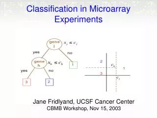
Classification Trees • Partition the feature space into a set of rectangles, then fit a simple model in each one • Binary tree structured classifiers are constructed by repeated splits of subsets (nodes) of the measurement space X into two descendant subsets (starting with X itself) • Each terminal subset is assigned a class label; the resulting partition of X corresponds to the classifier
Three Aspects of Tree Construction • Split Selection Rule • Split-stopping Rule • Class assignment Rule Different approaches to these three issues (e.g. CART: Classification And Regression Trees, Breiman et al. (1984); C4.5 and C5.0, Quinlan (1993)).
Three Rules (CART) • Splitting: At each node, choose split maximizing decrease in impurity (e.g.Gini index, entropy, misclassification error) • Split-stopping: Grow large tree, prune to obtain a sequence of subtrees, then use cross-validation to identify the subtree with lowest misclassification rate • Class assignment: For each terminal node, choose the class minimizing the resubstitution estimate of misclassification probability, given that a case falls into this node
Other Classifiers Include… • Support vector machines (SVMs) • Neural networks • Logistic regression • Projection pursuit • Bayesian belief networks
Features • Feature selection • Automatic with trees • For DA, NN need preliminary selection • Need to account for selection when assessing performance • Missing data • Automatic imputation with trees • Otherwise, impute (or ignore)
Why select features? Leukemia, 3 class affymetrix chip Left: no feature selection Right: top 100 most variables genes Lymphoma, 3 class lymphochip Left: no feature selection Right: top 100 most variables genes
Explicit feature selection I One-gene-at-a-time approaches. Genes are ranked based on the value of a univariate test statistic such as: t- or F-statistic or their non-parametric variants (Wilcoxon/Kruskal-Wallis); p-value. Possible meta-parameters include the number of genes G or a p-value cut-off. A formal choice of these parameters may be achieved by cross-validation or bootstrap procedures.
Multivariate approaches. More refined feature selection procedures consider the joint distribution of the expression measures, in order to detect genes with weak main effects but possibly strong interaction. Bo & Jonassen (2002): Subset selection procedures for screening gene pairs to be used in classification Breiman (1999): ranks genes according to importance statistic define in terms of prediction accuracy. Note that tree building itself does not involve explicit feature selection. Explicit feature selection II
Implicit feature selection Feature selection may also be performed implicitly by the classification rule itself. In classification trees, features are selected at each step based on reduction in impurity and The number of features used (or size of the tree) is determined by pruning th tree using cross-validation. Thus, feature selection is inherent part of tree-building and pruning deals with overfitting. Shrinkage methods and adaptive distance function May be used for LDA and kNN.
Distance and Standardization Trees. Trees are invariant under monotone transformation of individual features (genes), e.g. standardization. They are not invariant to standardization of observations (normalization in microarray context). DA. Based on Mahalanobis distance of the observations from the class means. Thus , the classifiers are invariant to standardization of the variables (genes) but not observations. (arrays) k-NN. Related to deciding on distance function. affected by both, features and observations standardization.
Polychotomous classification • It may be advantageous to convert a K-class • classification problem (K > 2) into a series of • binary problems. • All pairwise binary classification problems. • Consider all binary classification problems: the • final predicted class is the class that is selected • often among all binary comparisons. • One-against-all binary classification problem • Application of K binary rules to a test case • yields K estimates of class probabilities. Choose • the class with the largest posterior.
Performance assessment Any classifier needs to be evaluated for its performance on the future samples. It is almost never the case in microarray studies that a large independent population-based collection of samples is available at the time of intial classifier-building phase. One needs to estimate future performance based on what is available: often the same set that is used to build the classifier.
Diagram of performance assessment Classifier Training set (CV) Learning set Performance assessment Classifier Training set (CV) Test set Test set Classifier
Performance assessment (I) • Resubstitution estimation: error rate on the learning set • Problem: downward bias • Test set estimation: divide cases in learning set into two sets, L1 and L2; classifier built using L1, error rate computed for L2. L1 and L2 must be iid. • Problem: reduced effective sample size
Performance assessment (II) • V-fold cross-validation (CV) estimation: Cases in learning set randomly divided into V subsets of (nearly) equal size. Build classifiers leaving one set out; test set error rates computed on left out set and averaged. • Bias-variance tradeoff: smaller V can give larger bias but smaller variance • Computationally intensive