Estimating expression differences in cDNA microarray experiments
Estimating expression differences in cDNA microarray experiments. Statistics 246, Spring 2002 Week 8, Lecture 1. Some motherhood statements. Important aspects of a statistical analysis include: Tentatively separating systematic from random sources of variation

Estimating expression differences in cDNA microarray experiments
E N D
Presentation Transcript
Estimating expression differences in cDNA microarray experiments Statistics 246, Spring 2002 Week 8, Lecture 1
Some motherhood statements Important aspects of a statistical analysis include: • Tentatively separating systematic from random sources of variation • Removing the former and quantifying the latter, when the system is in control • Identifying and dealing with the most relevant source of variation in subsequent analyses Only if this is done can we hope to make more or less valid probability statements
The simplest cDNA microarray data analysis problem is identifying differentially expressed genes using one slide • This is a common enough hope • Efforts are frequently successful • It is not hard to do by eye • The problem is probably beyond formal statistical inference (valid p-values, etc) for the foreseeable future….why? In the next two slides, genes found to be up- or down-regulated in an 8 treatment (Srb1 over-expression) versus 8 control comparison are indicated in red and green, respectivley. What do we see?
Matt Callow’s Srb1 dataset (#5). Newton’s and Chen’s single slide method
Matt Callow’s Srb1 dataset (#8). Newton’s, Sapir & Churchill’s and Chen’s single slide method
The second simplest cDNA microarray data analysis problem is identifying differentially expressed genes using replicated slides There are a number of different aspects: • First, between-slide normalization; then • What should we look at: averages, SDs, t-statistics, other summaries? • How should we look at them? • Can we make valid probability statements? A report on work in progress: begin with an example.
Apo AI experiment (Matt Callow, LBNL) Goal. To identify genes with altered expression in the livers of Apo AI knock-out mice (T) compared to inbred C57Bl/6 control mice (C). • 8 treatment mice and 8 control mice • 16 hybridizations: liver mRNA from each of the 16 mice (Ti , Ci ) is labelled with Cy5, while pooled liver mRNA from the control mice (C*) is labelled with Cy3. • Probes: ~ 6,000 cDNAs (genes), including 200 related to lipid metabolism.
Which genes have changed?When permutation testing possible 1. For each gene and each hybridisation (8 ko + 8 ctl), use M=log2(R/G). 2. For each gene form the t statistic: average of 8 ko Ms - average of 8 ctl Ms sqrt(1/8 (SD of 8 ko Ms)2 + (SD of 8 ctl Ms)2) 3. Form a histogram of 6,000 t values. 4. Do a normal q-q plot; look for values “off the line”. 5. Permutation testing (next lecture). 6. Adjust for multiple testing (next lecture).
What is a normal q-q plot? We have a random sample, say ti, i=1, …,n, which we believe might come from a normal distribution. If it did, then for suitable and , ((ti-)/), i=1,…n would be uniformly distributed on [0,1](why?), where is the standard normal c.d.f.. Denoting the order statistics of the t-sample by t(1) ,t(2) ,….,t(n)we can then see that ((t(i) -)/) should be approximately i/n (why?). With this in mind, we’d expect t(i) to be about -1(i/n) + (why?). Thus if we plot t(i) against -1((i+1/2/(n+1)), we might expect to see a straight line of slope about with intercept about . (The 1/2 and 1 in numerator and denominator of the i/n are to avoid problems at the extremes.) This is our normal quantile-quantile plot, the i/n being a quantile of the uniform, and the -1being that of the normal.
Why a normal q-q plot? One of the things we want to do with our t-statistics is roughly speaking, to identify the extreme ones. It is natural to rank them, but how extreme is extreme? Since the sample sizes here are not too small ( two samples of 8 each gives 16 terms in the difference of the means), approximate normality is not an unreasonable expectation for the null marginal distribution. Converting ranked t’s into a normal q-q plot is a great way to see the extremes: they are the ones that are “off the line”, at one end or another. This technique is particularly helpful when we have thousands of values. Of course we can’t expect all differentially expressed genes to stand out as extremes: many will be masked by more extreme random variation, which is a big problem in this context. See next lecture for a discussion of these issues.
Gene annotation Apo AI EST, weakly sim. to STEROL DESATURASE CATECHOL O-METHYLTRANSFERASE Apo CIII EST, highly sim. to Apo AI EST Highly sim. to Apo CIII precursor similar to yeast sterol desaturase
Which genes have changed?Permutation testing not possible Our current approach is to use averages, SDs, t-statistics and a new statistic we call B, inspired by empirical Bayes. We hope in due course to calibrate B and use that as our main tool. We begin with the motivation, using data from a study in which each slide was replicated four times.
Points to note One set (green) has a high average M but also a high variance and a low t. Another (pale blue) has an average M near zero but a very small variance, leading to a large negative t. A third (dark blue) has a modest average M and a low variance, leading to a high positive t. A fourth (purple) has a moderate average M and a moderate variance, leading to a small t. Another pair (yellow, red) have moderate average Ms and middling variances, and moderately large ts. Which do we regard most favourably? Let’s look at M and t jointly.
M • t • t M Sets defined by cut-offs: from the Apo AI ko experiment
M • t • t M Results from the Apo AI ko experiment
M • t • t M Apo AI experiment: t vs average A.
T • B • t M B • t B Results from SR-BI transgenic experiment
M • B • t • M B • t B • t MB Results from SR-BI transgenic experiment
An empirical Bayes story Using average M alone, we ignore useful information in the SD across replicated. Some large values are large because of outliers. Using t alone, we are liable to be misled by very small SDs. With thousands of genes, some SDs will be very small. Formal testing can sort out these issues for us, but if we simply want to rank, what should we rank on? One approach (SAM) is to inflate the SDs slightly. Another approach can be based on the following empirical Bayes story. There are a number of variants. Suppose that our M values are independently and normally distributed, and that a proportion p of genes are differentially expressed, i.e. have M’s with non-zero means. Further, suppose that the variances and means of these are chosen jointly from inverse chi-square and normal conjugate priors, respectively. Genes not differentially expressed have zero means and variances from the same inverse chi-squared distribution. The scale and d.f. parameters in the inverse chi-square are estimated from the data, as is a parameter c connecting the prior for the mean with that for the variances. We then look for the posterior probability that a given gene is differentially expressed, and find it is an increasing function of B over the page. Details in the paper cited.
Empirical Bayes log posterior odds ratio (LOR) Notice that for large n this approximately t=M./s .
M • B • t • M B • t B • t M B Results from SR-BI transgenic experiment
M • B • t • M B • t B • t M B Results from SR-BI transgenic experiment
Comparison of different criteria These data come from the Srb1 transgenic mouse experiment with 8 replicates. See Table on next page. These data come from a mouse experiment with 8 replicates. See Table 1.
M. T B Comment . 0 0 0 Not differentially expressed genes. 0 0 1 False negatives in M. And T (high but not extreme) - detected by B. False positives in T - small M. but tiny variance. 0 1 0 0 1 1 False negatives in M., but detected by T and B. False positives in M. - Large M. but too large variance to be trusted. 1 0 0 1 0 1 False negatives i T - large M. and true moderately high variance. 1 1 0 No genes here - extreme for M. and T => extreme for B! 1 1 1 High in all three statistics - clearly differentially expressed. Table Sets of genes. ”1” indicates that the genes in the set are extreme* for that statistic. *|M.|>0.5 |T|>4.5 B>-2 These limits are chosen for illustratory reasons. Normally they would be slightly higher.
Extensions include dealing with • Replicates within and between slides • Several effects: use a linear model • ANOVA: are the effects equal? • Time series: selecting genes for trends
Summary (for the second simplest problem) • Microarray experiments typically have thousands of genes, but only few (1-10) replicates for each gene. • Averages can be driven by outliers. • ts can be driven by tiny variances. • B = LOR will, we hope • use information from all the genes • combine the best of M. and t • avoid the problems of M. and t Ranking on B could be helpful.
Use of linear models with cDNA microarray data In many situations - we met one with the olfactory bulb experiment back in Week 2 - we want to combine data from different experiments in a slightly more elaborate manner than simply averaging. One way of doing so is via (fixed effects) linear models, where we estimate certain quantities of interest which we call effects for each gene on our slide. Typically these estimates may be regarded as approximately normally distributed with common SD, and mean zero in the absence of any relevant differential expression. In such cases, the preceding two strategies: q-q plots, and various combinations of estimated effect (cf M.), standardized estimate (cf. t) both apply. We illustrate in a couple of cases.
Factorial design m m+a Different ways of estimating parameters. e.g. Zeffect. 1 = (m + z) - (m) = z 2 - 5 = ((m + a) - (m)) -((m + a)-(m + z)) = (a) - (a + z) = z 4 + 3 - 5 =…= z 2 P01 A1 4 1 3 5 P04 A 4 m+z m+z+a+za How do we combine the information?
Regression analysis Define a matrix X so that E(M)=X Use least squares estimate for z, a, za
Estimates of zone effects log(zone 4 / zone1) vs ave A gene A gene B = average log√(R*G)
Estimates of zone effects vs SE Z effect • • t = / SE • t Log2(SE)
Estimates of age effects vs estimates of zone effects Zone Age Zone Age
Top 50 genes from each effect Zone . Age interaction Age 19 0 48 29 2 0 19 Zone
UCB/WEHI Yee Hwa Yang Sandrine Dudoit Ingrid Lönnstedt Natalie Thorne David Freedman Ngai lab, UCB Matt Callow (LBNL) Acknowledgments
Some web sites: Technical reports, talks, software etc. http://www.stat.berkeley.edu/users/terry/zarray/Html/ Statistical software R “GNU’s S” http://lib.stat.cmu.edu/R/CRAN/ Packages within R environment: -- Spot http://www.cmis.csiro.au/iap/spot.htm -- SMA (statistics for microarray analysis) http://www.stat.berkeley.edu/users/terry/zarray/Software /smacode.html