Download
1 / 60
600 likes | 719 Vues
This lecture provides an in-depth introduction to transcriptional networks, focusing on gene regulatory mechanisms. It discusses methodologies such as microarray experiments, MA plots, and normalization techniques for gene expression data. Various tests for differential gene expression and the importance of multiple testing and FDR are also covered. A case study on the hierarchical structure of transcriptional regulatory networks in *Escherichia coli* highlights the interplay of regulatory genes and the identification of network motifs through data integration from multiple sources.

E N D
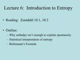
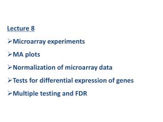
Lecture 6 • Introduction to transcriptional networks • Microarray experiments • MA plots • Normalization of microarray data • Tests for differential expression of genes • Multiple testing and FDR
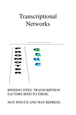
transcriptional networks By the term transcriptional networks we generally mean gene regulatory networks Unlike protein-protein interaction networks the transcriptional networks are directed networks
transcriptional networks: Basic mechanism of gene regulation
transcriptional networks Most genes are regulated at transcription level and it is assumed that 5-10% of protein coding genes encode regulatory proteins. Some regulatory proteins play targeted role i.e. they take part in regulation of a few genes. Some regulatory proteins play more general role in initiating transcription (for example the eukaryotic transcription factors of type II or the RNA polymerase itself that is essential for the transcription of all genes). It is considered that dedicated regulatory proteins are those that affect up to 5% genes of a genome. However the boundary between the generalist and dedicated regulatory proteins is blurred.
transcriptional networks • Experiments and methods used to generate data to determine regulatory relations • Complementary DNA microarrays • Oligonucleotide chips • Reverse transcription polymerase chain reaction • Serial analysis of gene expression • Chromatin Immunoprecipitation • Next generation sequencing • Bioinformatics—e.g. by way of identifying binding sites
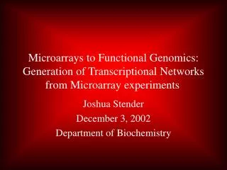
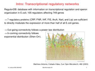
Transcriptional Networks: Case study 1 • An extended transcriptional regulatory network of Escherichia coli and analysis of its hierarchical structure and network motifs • Hong-Wu Ma, Bharani Kumar, Uta Ditges2, Florian Gunzer2, Jan Buer1,2 and An-Ping Zeng* • Nucleic Acids Research, 2004, Vol. 32, No. 22 6643–6649 • This work combined data sets from 3 different sources: • RegulonDB (version 4.0, http://www.cifn.unam.mx/Computational_Genomics/regulondb/) • Ecocyc (version 8.0, www.ecocyc.org) • Shen-Orr,S.S., Milo,R., Mangan,S. and Alon,U. (2002) Network motifs in the transcriptional regulation network of Escherichia coli. Nature Genet., 31, 64–68.
Transcriptional Network: Case study 1 Nucleic Acids Research, 2004, Vol. 32, No. 22 6643–6649 Comparison of the TRN of E.coli from three different data sources (A) Based on number of genes (B) Based on number regulatory interactions
Transcriptional Network: Case study 1 Nucleic Acids Research, 2004, Vol. 32, No. 22 6643–6649 A combined network that includes all the 2624 interactions from the three data sets has been produced. In addition, this work extended this network by adding 23 additional genes and around 100 regulatory relationships through literature survey. The final TRN altogether includes 1278 genes and 2724 interactions.
Transcriptional Network: Case study 1 Nucleic Acids Research, 2004, Vol. 32, No. 22 6643–6649 • This work discovered a hierarchical structure in the TRN. • The hierachical structure was identified according to the following way: • genes which do not code for transcription factors (TFs) or code for a TF which only regulates its own expression (auto-regulatory loop) were assigned to layer 1 (the lowest layer); • then we removed all the genes in layer 1 and from the remaining network identified TFs which do not regulate other genes and assigned the corresponding genes in layer 2; • we repeated step 2 to remove nodes which have been assigned to a layer and identified a new layer until all the genes were assigned to different layers. As a result, a nine layer hierarchical structure was uncovered. From BMC Bioinformatics 2004, 5:199 of the related authors
Transcriptional Network: Case study 1 Nucleic Acids Research, 2004, Vol. 32, No. 22 6643–6649
Transcriptional Network: Case study 1 Nucleic Acids Research, 2004, Vol. 32, No. 22 6643–6649 The hierarchical structure implies absence of cycles in the network i.e. feedback loops (though auto regulatory and inter-regulatory loops exist) As the network is not complete, we cannot say that feedback loop could not be found in future however it seems they would not be too many. A possible biological explanation for the existence of this hierarchical structure is that the interactions in this particular TRN are between proteins and genes without involving metabolites. Only after a regulating gene has been transcribed, translated and eventually further modified by cofactors or other proteins, it can regulate the target gene. A feedback from the regulated gene at transcriptional level may delay the process for the target gene to access a desired expression level in a new environment.
Transcriptional Network: Case study 1 Nucleic Acids Research, 2004, Vol. 32, No. 22 6643–6649 Feedback control may be mainly through other interactions (e.g. metabolite and protein interaction) at post-transcriptional level rather than through transcriptional interactions between proteins and genes. For example, a gene at the bottom layer may code for a metabolic enzyme, the product of which can bind to a regulator which in turn regulates its expression. In this case, the feedback is through metabolite–protein interaction to change the activity of the transcription factor and then to affect the expression of the regulated gene. Therefore, to fully understand the gene expression regulation, an integrated network that includes different interactions is needed.
Transcriptional Network: Case study 1 Nucleic Acids Research, 2004, Vol. 32, No. 22 6643–6649 To calculate network motifs in the E.coli TRN, this work removed all the loops in the network (including the autoregulatory loops and the two-gene regulatory loops). Then they used the program Mfinder developed by Kashtan et al. to generate the motif profiles. The first four types are the so-called coherent FFLs in which the direct effect of the up regulator is consistent with its indirect effect through the mid regulator. In contrast, the last four types of FFLs are incoherent because the direct effect of the up regulator is contradictive with its indirect effect
Transcriptional Network: Case study 1 Nucleic Acids Research, 2004, Vol. 32, No. 22 6643–6649 (A) Gene gadA is regulated by six FFLs (B)Gene lpd is regulated by five FFLs (C) Gene slp is regulated by 17 regulators
Transcriptional Network: Case study 1 Nucleic Acids Research, 2004, Vol. 32, No. 22 6643–6649
DNA Microarray Typical microarray chip • Though most cells in an organism contain the same genes, not all of the genes are used in each cell. • Some genes are turned on, or "expressed" when needed in particular types of cells. • Microarray technology allows us to look at many genes at once and determine which are expressed in a particular cell type.
DNA Microarray Typical microarray chip • DNA molecules representing many genes are placed in discrete spots on a microscope slide which are called probes. • Messenger RNA--the working copies of genes within cells is purified from cells of a particular type. • The RNA molecules are then "labeled" by attaching a fluorescent dye that allows us to see them under a microscope, and added to the DNA dots on the microarray. • Due to a phenomenon termed base-pairing, RNA will stick to the probe corresponding to the gene it came from
DNA Microarray Usually a gene is interrogated by 11 to 20 probes and usually each probe is a 25-mer sequence The probes are typically spaced widely along the sequence Sometimes probes are choosen closer to the 3’ end of the sequence A probe that is exactly complementary to the sequence is called perfect match (PM) A mismatch probe (MM) is not complementary only at the central position In theory MM probes can be used to quantify and remove non specific hybridization Source: PhD thesis by Benjamin Milo Bolstad, 2004, University of California, Barkeley
Sample preparation and hybridization Source: PhD thesis by Benjamin Milo Bolstad, 2004, University of California, Barkeley
Sample preparation and hybridization During the hybridization process cRNA binds to the array Earlier probes had all the probes of a probset located continuously on the array This may fall prey to spatial defects Newer chips have all the probes spread out across the array A PM and MM probe pair are always adjacent on the array Source: PhD thesis by Benjamin Milo Bolstad, 2004, University of California, Barkeley
Growth curve of bacteria • Samples can be taken at different stages of the growth curve • One of them is considered as control and others are considered as targets • Samples can be taken before and after application of drugs • Sample can be taken under different experimental conditions e.g. starvation of some metabolite or so • What types of samples should be used depends on the target of the experiment at hand.
DNA Microarray Typical microarray chip • After washing away all of the unstuck RNA, the microarray can be observed under a microscope and it can be determined which RNA remains stuck to the DNA spots • Microarray technology can be used to learn which genes are expressed differently in a target sample compared to a control sample (e.g diseased versus healthy tissues) • However background correction and normalization are necessary before making useful decisions or conclusions
MA plots MA plots are typically used to compare two color channels, two arrays or two groups of arrays The vertical axis is the difference between the logarithm of the signals(the log ratio) and the horizontal axis is the average of the logarithms of the signals The M stands for minus and A stands for add MA is also mnemonic for microarray Mi= log(Xij) - log(Xik) = Log(Xij/Xik) (Log ratio) Ai=[log(Xij) + log(Xik)]/2 (Average log intensity)
A typical MA plot From the first plot we can see differences between two arrays but the non linear trend is not apparent This is because there are many points at low intensities compared to at high intensities MA plot allows us to assess the behavior across all intensities
Normalization of microarray data Normalization is the process of removing unwanted non-biological variation that might exist between chips in microarray experiments By normalization we want to remove the non-biological variation and thus make the biological variations more apparent.
Normalization within individual arrays Sij = Xij- Xj Scaling: Cij= ( Xij- Xj ) / σj Centering:
Effect of Scaling and centering normalization Original Data Centering Scaling Mean = 0 Standard deviation = 1 Mean = 0
Normalization between a pair of arrays: Loess(Lowess) Normalization Lowess normalization is separately applied to each experiment with two dyes This method can be used to normalize Cy5 and Cy3 channel intensities (usually one of them is control and the other is the target) using MA plots
Normalization between a pair of arrays: Loess(Lowess) Normalization 2 channel data Mi=Log(Ti/Ci) (Log ratio) Ai=[log(Ti) + log(Ci)]/2 (Average log intensity) Mi=Log(Ti/Ci) Each point corresponds to a single gene Ai=[log(Ti) + log(Ci)]/2
Typical regression line Normalization between a pair of arrays: Loess(Lowess) Normalization Mi=Log(Ti/Ci) (Log ratio) Ai=[log(Ti) + log(Ci)]/2 (Average log intensity) Each point corresponds to a single gene Mi=Log(Ti/Ci) The MA plot shows some bias Ai=[log(Ti) + log(Ci)]/2
Normalization between a pair of arrays: Loess(Lowess) Normalization Mi=Log(Ti/Ci) (Log ratio) Ai=[log(Ti) + log(Ci)]/2 (Average log intensity) Each point corresponds to a single gene Mi=Log(Ti/Ci) The MA plot shows some bias Usually several regression lines/polynomials are considered for different sections Ai=[log(Ti) + log(Ci)]/2 The final result is a smooth curve providing a model for the data. This model is then used to remove the bias of the data points
Normalization between a pair of arrays: Loess(Lowess) Normalization Bias reduction by lowess normalization
Normalization between a pair of arrays: Loess(Lowess) Normalization Unnormalized fold changes fold changes after Loess normalization
Normalization across arrays Here we are discussing the following two normalization procedure applicable to a number of arrays • Quantile normalization • Baseline scaling normalization
Normalization across arrays Quantile normalization The goal of quantile normalization is to give the same empirical distribution to the intensities of each array If two data sets have the same distribution then their quantile- quantile plot will have straight diagonal line with slope 1 and intercept 0. Or projecting the data points of the quantile- quantile plot to 45-degree line gives the transformation to have the same distribution. quantile- quantile plot motivates the quantile normalization algorithm
Normalization across arrays Quantile normalization Algorithm Source: PhD thesis by Benjamin Milo Bolstad, 2004, University of California, Barkeley
Normalization across arrays QuantileNormalization: Original data Sort 1. Sort each column of X (values) 2. Take the means across rows of X sort Sort 3. Assign this mean to each element in the row to get X' sort 4. Get X normalized by rearranging each column of X' sort to have the same ordering as original X
Normalization across arrays Raw data After quantile normalization
Normalization across arrays Baseline scaling method In this method a baseline array is chosen and all the arrays are scaled to have the same mean intensity as this chosen array This is equivalent to selecting a baseline array and then fitting a linear regression line without intercept between the chosen array and every other array
Normalization across arrays Baseline scaling method
Normalization across arrays Raw data After Baseline scaling normalization
Tests for differential expression of genes Let x1…..xn and y1…yn be the independent measurements of the same probe/gene across two conditions. Whether the gene is differentially expressed between two conditions can be determined using statistical tests.
Tests for differential expression of genes • Important issues of a test procedure are • Whether the distributional assumptions are valid • Whether the replicates are independent of each other • Whether the number of replicates are sufficient • Whether outliers are removed from the sample • Replicates from different experiments should not be mixed since they have different characteristics and cannot be treated as independent replicates
Tests for differential expression of genes Most commonly used statistical tests are as follows: (a) Student’s t-test (b) Welch’s test (c) Wilcoxon’s rank sum test (d) Permutation tests The first two test assumes that the samples are taken from Gaussian distributed data and the p-values are calculated by a probability distribution function The later two are nonparametric and the p values are calculated using combinatorial arguments.
Student’s t-test Assumptions: Both samples are taken from Gaussian distribution that have equal variances Degree of freedom: m+n-2 Welch’s test is a variant of t-test where t is calculated as follows Welch’s test does not assume equal population variances
Student’s t-test The value of t is supposed to follow a t-distribution. After calculating the value of t we can determine the p-value from the t distribution of the corresponding degree of freedom