Download
1 / 262
2.66k likes | 2.79k Vues
Dive into the fascinating world of GPS technology, from its historical roots to the intricate signal frequencies and measurements used today. Discover how GPS works and its role in navigation and positioning systems.

E N D
Introduction to GPS • “… it isn’t hard to operate a GPS receiver – matter of fact, most of them are so user-friendly you don’t need to know the first thing about GPS to make them work; that is, until they don’t. Getting coordinates from a GPS receiver is usually a matter of pushing buttons, but knowing what those coordinates are, and more importantly, what they aren’t, is more difficult.” Jan Van Sickle
Use of Satellites in Surveying • Started as early as Sputnik (1957) • Continued with other satellites • Measuring positions of satellites against background stars on photographs • Laser ranging • Used Doppler effect to determine velocity vector
TRANSIT Satellite • Navy Navigation Satellite System (NNSS) started in 1960s • Used the Doppler shift of the signal to determine velocity vector • Six satellites in low (1100 km) circular, polar orbits • One satellite every 90 minutes, need 2 passes • Susceptible to atmospheric drag and gravitational perturbations • Poor quality orbital parameters • Produces poor positions (by modern standards)
Brief History of GPS • Initial work in 1970s • Counselman, Shapiro, etc. (MIT) • First used for practical purposes in 1980s • Civilian use ahead of military use • Initial operational capability (IOC) July ‘93 • Full operational capability (FOC) 17 July 1995
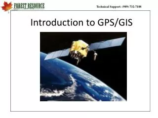
GPS Overview • Consists of ~24 satellites • 4 satellites in 6 orbital planes • Planes inclined 55° • 20,000 km orbits • Periods of 11h 58m • Each satellite carries multiple atomic clocks
GPS Segments • User Segment • Military and civilian users • Space Segment • 24 satellite constellation • Control Segment • Worldwide network of stations
Space Segment • Block I • Block II • Block IIA (A – advanced) • Block IIR (R – replenishment) • Block IIF (F – Follow on) • Block III • See http://www.spaceandtech.com/spacedata/constellations/navstar-gps-block1_conspecs.shtml
Control Segment • Worldwide network of stations • Master Control Station – Colorado Springs, CO • Monitoring Stations – Ascension Island, Colorado Springs, Diego Garcia, Hawaii, Kwajalein • Other stations run by National Imagery and Mapping Agency (NIMA) • Ground Control Stations – Ascension, Diego Garcia, Kwajalein
USNO USNO AMC Data Flow Satellite Signal Timing data Control Timing Links Satellite Signal Master Control Station Data Monitor Station Time
Basic Idea • Broadcast signal has time embedded in it • Need to determine distance from satellite to receiver • One way uses distance = velocity * time • If time between when the signal is sent and when it is received is known, then distance from satellite is known • Using multiple distances, location can be determined (similar to trilateration)
GPS Signal Frequency • Fundamental Frequency 10.23MHz (f0) • 2 Carrier Frequencies • L1 (1575.42 MHz) (154 f0) • L2 (1227.60 MHz) (120 f0) • 3 Codes • Coarse Acquisition (C/A) 1.023 MHz • Precise (P) 10.23 MHz • Encrypted (Y) • Spread Spectrum • Harder to jam
Codes • Stream of binary digits known as bits or chips • Sometimes called pseudorandom noise (PRN) codes • Code state +1 and –1 • C/A code on L1 • P code on L1 and L2 • Phase modulated
C/A Code • 1023 binary digits • Repeats every millisecond • Each satellite assigned a unique C/A-code • Enables identification of satellite • Available to all users • Sometimes referred to as Standard Positioning Service (SPS) • Used to be degraded by Selective Availability (SA)
P Code • 10 times faster than C/A code • Split into 38 segments • 32 are assigned to GPS satellites • Satellites often identified by which part of the message they are broadcasting • PRN number • Sometimes referred to as Precise Positioning Service (PPS) • When encrypted, called Y code • Known as antispoofing (AS)
Future Signal • C/A code on L2 • 2 additional military codes on L1 and L2 • 3rd civil signal on L5 (1176.45 MHz) • Better accuracy under noisy and multipath conditions • Should improve real-time kinematic (RTK) surveys
Time Systems • Each satellite has multiple atomic clocks • Used for time and frequency on satellite • GPS uses GPS Time • Atomic time started 6 January 1980 • Not adjusted for leap seconds • Used for time tagging GPS signals • Coordinated Universal Time (UTC) • Atomic time adjusted for leap seconds to be within ±0.9 s of UT1 (Earth rotation time)
Pseudorange Measurements • Can use either C/A- or P-code • Determine time from transmission of signal to when the signal is received • Distance = time*speed of light • Since the position of the satellite is assumed to be known, a new position on the ground can be determined from multiple measurements
Carrier-phase Measurements • The range is the sum of the number of full cycles (measured in wavelengths) plus a fractional cycle • ρ = N*λ + n* λ • The fraction of a cycle can be measured very accurately • Determining the total number of full cycles (N) is not trivial • Initial cycle ambiguity • Once determined, can be tracked unless …
Cycle Slips • Discontinuity or jump in phase measurements • Changes by an integer number • Caused by signal loss • Obstructions • Radio interference • Ionospheric disturbance • Receiver dynamics • Receiver malfunction
How to Fix Cycle Slips? • Slips need to be detected and fixed • Triple differences can aid in cycle slips • Will only affect one of the series • Should stand out • Once detected, it can be fixed
GPS Errors and Biases • Satellite Errors • Potentially different for each satellite • Transmission Errors • Depends on path of signal • Receiver Errors • Potentially different for each receiver
Linear Combination • Errors and biases, which cannot be modeled, degrade the data • Receivers that are ‘close enough’ have very similar errors and biases • Data can be combined in ways to mitigate the effects of errors and biases
Linear Combination • Combine data from two receivers to one satellite • Should have same satellite and atmospheric errors • Differences should cancel these effects out
Linear Combination • Combine data from one receiver to two satellites • Should have same receiver and atmospheric errors • Differences should cancel these effects out
Linear Combination • Combine data from two receivers to two satellites • Should have same receiver, satellite and atmospheric errors • Differences should cancel out
Linear Combination • Can also combine the L1 and L2 data to eliminate the effects of the ionosphere • Ionosphere-free combination • L1 and L2 phases can also be combined to form the wide-lane observable • Long wavelength • Useful in resolving integer ambiguity
Two Reference Frames • Satellites operate in an inertial reference frame • Best way to handle the laws of physics • Receivers operate in a terrestrial reference frame • Sometimes called an Earth-centered, Earth-fixed (ECEF) frame • Best way to determine positions
Inertial Frame (Historically) • X axis through the vernal equinox • Y axis is 90° to the ‘east’ • Z axis through the Earth’s angular momentum axis • X-Y plane is the celestial equator • Z axis is through the celestial North Pole
Inertial Frame From http://celestrak.com/columns/v02n01/
Inertial Frame • Defined by the positions of distant radio sources called quasars • Realization from observations provided by Very Long Baseline Interferometry (VLBI) • e.g. International Celestial Reference Frame • Right-handed, Cartesian coordinate system
Terrestrial Frame (Historically) • X axis through the Greenwich meridian • Y axis is 90° to the east • Z axis through the Earth’s angular momentum axis • X-Y plane is the equator • Z axis is through the North Pole
Terrestrial Frame From http://www.nottingham.ac.uk/iessg/coord1.htm
Terrestrial Frame • Defined by the positions of reference points • Realization from observations provided by VLBI, SLR, and GPS • e.g. International Terrestrial Reference Frame • e.g. World Geodetic System (WGS)-84 • Right-handed, Cartesian coordinate system
Terrestrial Frame • Can transform from non-Cartesian (geodetic) coordinates to Cartesian coordinates • X = (N+h) cosφ cosλ • Y = (N+h) cosφ sinλ • Z = [ N(1-e2)+h] sin φ • Where N = a/sqrt(1-e2sin2 φ) • h = ellipsoid height • φ = latitude • λ = longitude
Transformation between Frames • Transformation is accomplished through rotation by Earth orientation parameters (EOPs) • Polar Motion (W) • Earth rotation (T) • Precession/nutation (P)(N) • xcts = (W)(T)(N)(P)xcis
Datums • Based on a reference ellipsoid • Semimajor axis (a) and semiminor axis (b) or semimajor axis (a) and flattening (f) • Needs to have a well defined center (origin) • Needs to have a well defined direction or axes (orientation)
Datums • Can be done with 8 parameters • 2 define the ellipsoid • 3 define the origin of the ellipsoid • 3 define the orientation of the ellipsoid
Datums • North American Datum 1927 (NAD27) • Clarke ellipsoid of 1866 • North American Vertical Datum 1929 (NAVD29) • North American Datum 1983 (NAD83) • GRS 1980 ellipsoid • North American Vertical Datum 1988 (NAVD88) • Even the last two have minimal input from GPS
Vertical Measurements • Vertical measurements from GPS are relative to the ellipsoid (ellipsoid height) • Not from the geoid or topography • To translate to other surfaces (either reference or real) requires additional information • Orthometric or geoid heights
Vertical Surfaces From http://www.butterworth.uk.com/geodesy.html
HARN • High Accuracy Reference Network (HARN) • Created by states, with federal assistance (NGS) • Predominantly based on GPS observations • Very accurate
Plane Coordinate Systems • Used over ‘local’ areas • State Plane Coordinate (SPC) systems • Results of projection onto surface • Lambert conic projection • Mercator (cylindrical) projection
Time Systems • Earth rotation time • Solar/sidereal • Dynamical • Barycenter/terrestrial • Atomic (off by integer seconds) • Coordinated Universal Time (UTC) • International Atomic Time (TAI) • GPS Time