Input-Output Accounts
Module-I: PP3.2. Input-Output Accounts. Training Course Material for e-Library on System of National Accounts March 2009. Outline. Input-Output Models Input-Output (IO) System Construction of IO Tables Related concepts of IO Account. Input-Output Models.

Input-Output Accounts
E N D
Presentation Transcript
Module-I: PP3.2 Input-Output Accounts Training Course Material for e-Library on System of National Accounts March 2009
Outline • Input-Output Models • Input-Output (IO) System • Construction of IO Tables • Related concepts of IO Account
Input-Output Models Capture inter-industry transactions: • Industries use the products of other industries to produce their own products • For example - automobile producers use steel, glass, rubber, and plastic products to produce automobiles. • Outputs from one industry become inputs to another • When you buy a car, you affect the demand for glass, plastic, steel, etc.
Tires Glass Plastic Other Components Steel Basic Input-Output Logic Automobile Factory
Individual Consumers School Districts Trucking Companies Automobile Factory From the Tire Producer’s Perspective FINAL DEMAND FOR TIRES Tire Factory INTER- MEDIATE DEMAND FOR TIRES
$$ Consumption Spending (Yi) Goods & Services Businesses Households Labor $$ Wages & Salaries Simplified Circular Flow Businesses Businesses purchase from other businesses to produce their own goods / services. This is intermediate demand or Xij (output of industry i sold to industry j) Households buy the output of business: final demand or Yi Households sell labor & other inputs to business as inputs to production
Input Output Account • Extensive Desegregation of Production Account: products / commodities produced, industries and other activities shown separately • Products /Commodities are goods and services normally intended for sale in market at a price that covers cost of production • Industries are productive units producing Products • Activities consists of industries, producers of government services and producers of private non-profit services to households
Input Output System Three Basic Elements I: Classifies economy into productive sectors (industries), say, n II: Considers both uses--Intermediate and Final III: Considers availability of a product with time dimension
Input Output System(Contd.)The Balance equation • Availability of a product = Utilization of the product • Opening Stock+ Current Production + Import = Intermediate Use+ Consumption +FCF +Export +Closing Stock Or, • Intermediate Use + Consumption + FCF + Export -Imports +Change in Stock (Closing-Opening) = Current Production
Denote, Xij : Output of ith Product used as input in jth industry Xi : Output of the ithProduct Ci : Consumption of the ithProduct Fi : Fixed Capital Formation of the ithProduct Ei : Export of the ithProduct Mi : Import of the ithProduct Si : Change in stock of the ithProduct
Using notations, the balance equation is, Xi1 + Xi2 + ……..Xin + Ci+ Fi + Ei - Mi + Si = Xi Or, Xi1 + Xi2 + ……..Xin + Yi = Xi , i =1,2,…n Where, Yi = Ci+ Fi + Ei - Mi + Si (final use of ith product) When we write the above n equations one below the other, a form of table appears This table when written along with the primary inputs (gross value added) row placed exactly below the first n elements of the equation, we see square Input-Output Table
Leontief Open Static Model Xi1 + Xi2 + ……..Xin + Yi = Xi , i =1,2,…n Define, aij = Xij / Xj , Thus, Xi = j Xij + Yi = j aij Xj + Yi where, Xij = aij Xj X=AX+Y, (I-A)X=Y, X = (I-A)-1 Y It is the Leontief Open Static Model
What does Input Output Table show? • I-O table is a statistical description in a matrix form that shows the transactions of goods and services (products) by industries to various industries (inter-industry) and final users • I-O table shows how an industry obtains various material inputs needed by it to produce its output from various industries and how it produces its output making use of the material and primary inputs
I-O Transactions Table Table 1
I-O Flow Table (contd.) • The rows of the table above represent the allocation of a given sector, partly going to intermediate demand, and partly to final demand • The column show intermediate inputs and primary inputs used in each sector for production of output • Based on the matrix system, it shows that each cell of the I-O table plays a double role: • for example x12, if it goes along the row, x12 represents amount of output of sector 1 used by sector 2 as intermediate input. At the same time, if it is down the column, x12 represents an input of sector 2 acquired from sector 1
I-O Flow Table (contd.) • The output allocation of each sectors can be written down in algebraic equation as : x11 + x12 + x13 + Y1 = X1 x21 + x22 + x23 + Y2 = X2 …..(1.1) x31 + x32 + x33 + Y3 = X3 • The input of all sectors may also be written down in algebraic equations as : x11 + x21 + x31 + V1 = X1 x12 + x22 + x32 + V2 = X2 …..(1.2) x13 + x23 + x33 + V3 = X3
I-O Flow Table (contd.) Table 2
I-O Coefficient Table Table 3 Where : aij = Xij / Xj
I-O Coefficient Table (contd.) • Table 3 above can be written down in algebraic equations as : a11x1 + a12x2 + a13x3 + Y1 = X1 a21x1 + a22x2 + a23x3 + Y2 = X2 …..(1.3) a31x1 + a32x2 + a33x3 + Y3 = X3 • In matrix form, equation 1.3 can be written as follows : • Or is usually written in matrix form as : AX + Y = X ……(1.5) Where : A is coefficient matrix X is vector of output Y is vector of final demand X + = ….(1.4) a11 a12 a13 a21 a22 a23 a31 a32 a33 X1 X2 X3 Y1 Y2 Y3 X1 X2 X3
I-O Coefficient Table (contd.) Table 4
The Inverse Matrix • The inverse matrix can be calculated when the A matrix is known • The inverse matrix can be calculated from the equation 1.5 as follows : AX + Y = X X – AX = Y ……(1.6) ( I – A ) X = Y X = ( I – A )-1 Y Where : I is identity matrix ( I – A )-1 is inverse matrix (Leontief inverse)
The Inverse Matrix (contd.) • For illustration, the inverse matrix of (I-A)-1is obtained in following steps
Method of Construction of Input-Output Transactions Table • Make matrix and Absorption matrix • Furnish the basic info for an IOTT either on product group basis or industry group basis • Absorption matrix consists of three main parts: • (i) products analysis of purchase of intermediate goods and services by industry groups, i.e., input flow • (ii) products analysis of purchase by final users, i.e., final demand, and • (iii) analysis of primary inputs into the industry consisting of wage and non-wage income
Make Matrixis the output matrix of products and by products (at basic prices). Rows represent industry groups and columns represent Product groups
Product x Product table is suitable for Product planning • Industry x industry table is suitable for industry planning. • The pure matrices, Product x Product and industry x industry can be obtained by matrix operations under certain assumptions, namely • Industry Technology Assumption • Commodity / Product Technology Assumption • A mixed one
Technology assumptionsFor Transferring output of secondary products • Industry Technology assumption is one where input structure of a secondary product is considered to be similar to that of the industry where it has been produced • Commodity (Product) Technology assumption is one where input structure of the secondary product is assumed to be similar to that of the industry where it is primarily produced
Notations X: Absorption matrix; M: Make matrix f: Final use of Products y: Primary incomes q: Outputs of Products g: Outputs of Industries B : Products x Industry coefficient matrix A : Products x Products coefficient matrix W: Products x Products flow matrix
From Make Matrix C : Product Mix Matrix : the columns of which show the proportions in which a particular industry produces various products, C=M' g*-1 D : Market Share Matrix: the columns of which show the proportions in which various industries produce the total output of a particular product D=M q*-1 q* , g* are diagonal matrices and so are their inverse
Denote further, E : Industry x Industry coefficient matrix Z : Industry x Industry flow matrix f : final use of products : Final use of the industry output mix
For Product x ProductTable under Commodity (Product) Technology Assumption, Inputs into industry j (bij ) comprise: the weighted average of inputs of each of the products which it produces, the weights being the proportions (cij ) in which industry j produces the various products, i.e., for illustration taking only three sectors, bij = ai1 c1j + ai2 c2j + ai3 c3j Thus B=AC , implying A= BC-1
For Product x Product Table under Industry Technology Assumption, Inputs into product j (aij) will be the weighted average of the inputs (bij) of each of the industries which produce product j , and weights will be market shares (dij) of each industry in the production of product j i.e., for illustration taking only three sectors, aij = bi1d1j + bi2d2j + bi3d3j Thus, A= BD
Planning Models For product analysis the model is q = A q + f Under product technology assumption q = (BC-1 ) q + f Under industry technology assumption q = (BD) q + f
Planning Models(Contd.) For industry analysis the model is g = E g + , Under product technology assumption g = (C-1 B) g + C-1 f , Under industry technology assumption g = (DB) g + D f ,