Mössbauer parameters from DFT-based WIEN2k calculations for extended systems

1. Mössbauer parameters from DFT-based WIEN2k calculations for extended systems Peter Blaha Institute of Materials Chemistry TU Vienna

2. Main Mössbauer parameters: • The main (conventional) Mössbauer spectroscopy parameters which we want to calculate by theory are: • Isomer shift: d = a (r0Sample – r0Reference); • it is proportional to the electron density r0at the nucleus • the constant a is proportional to the change of nuclear radii during the transition (we use a=-.291 au3mm s-1) • Magnetic Hyperfine fields: Btot = Bcontact + Borb + Bdip • these fields are proportional to the spin-density at the nucleus and the orbital moment of the probed atom as well as the spin moment distribution in the crystal • Quadrupole splitting: De Q Vzz • given by the product of the nuclear quadrupole moment Q times the electric field gradient Vzz. The EFG is proportional to an integral over the non-spherical charge density (weighted by 1/r3)

3. Schrödinger equation • From the previous slide it is obvious, that we need an accurate knowledge of the electron (and magnetization) density, which in principle can be obtained from the solution of the many-body Schrödinger equation in the corresponding solid. H Y = E Y • However, a many-body problem with ~1023 particles is not solvable at all and we must create models for the real material and rely on an approximate solution of the Schrödinger equation. (This will be briefly discussed in the next slides and my preferred options are marked in red.)

4. Concepts when solving Schrödingers-equation Treatment of spin Form of potential “Muffin-tin” MT atomic sphere approximation (ASA) pseudopotential (PP) Full potential : FP Non-spinpolarized Spin polarized (with certain magnetic order) Relativistic treatment of the electrons exchange and correlation potential Hartree-Fock (+correlations) Density functional theory (DFT) Local density approximation (LDA) Generalized gradient approximation (GGA) Beyond LDA: e.g. LDA+U non relativistic semi-relativistic fully-relativistic Schrödinger - equation Basis functions Representation of solid plane waves : PW augmented plane waves : APW atomic oribtals. e.g. Slater (STO), Gaussians (GTO), LMTO, numerical basis non periodic (cluster, individual MOs) periodic (unit cell, Blochfunctions, “bandstructure”)

5. Representation of the solid • cluster model: • approximate the solid by a finite (small) number of atoms. This can be a good approximation for “molecular crystals”. • periodic model: • use a “unit cell”, which is repeated infinitely. This approximates the “real” solid (finite with surfaces, imperfect) by an infinite “ideal” solid. • with “supercells” also surfaces, vacancies or impurities can be modelled. BaSnO3 SnS

6. Exchange and correlation • The electron-electron interaction can be approximated by: • Hartree-Fock • exact exchange, but no correlation at all (in solids often very important !) • correlation can approximately be added at various levels: MP2, CC, CI, ... • HF (and even more adding correlation) is very expensive in solids. • Density functional theory: • the exact functional is unknown, thus one must approximate exchange + correlation. Fast method, fairly accurate in solids. • LDA: local density approximation, “free electron gas” • GGA: generalized gradient approximation, various functionals • hybrid-DFT: mixing of HF + GGA, various functionals • LDA+U, DMFT: explicit (heuristic) inclusion of correlations • a brief summary of DFT follows

7. DFT Density Functional Theory Hohenberg-Kohn theorem: (exact) The total energy of an interacting inhomogeneous electron gas in the presence of an external potential Vext(r ) is a functional of the density  • This (exact) statement states, that we need to know only the • electron density r, but we do NOT need to know the • wavefunctions (solution of Schrödinger equation not necessary). • However, the exact functional form of F[r] is unknown and • any approximation so far is too crude.

8. DFT - Kohn Sham (still exact) Lets decompose the total functional F[r] into parts which can be calculated „exactly“ and some „unknown, but small“ rest: Ekinetic non interacting Ene EcoulombEee Exc exchange-correlation • Ekinetic is the kinetic energy of non-interacting particles • Ecoulomb is the “classical” electrostatic interaction between electrons • (including the self-interaction energy) • Exc is the exchange-correlation energy and should correct for the • self-interaction and approx. kinetic energy • The exact Exc is again unknown, but now an approximation for the • “small correction” may be accurate enough.

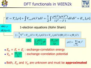
9. Kohn-Sham equations 1-electron equations (Kohn Sham) vary  -Z/r Excand Vxcare unknown and must be approximated LDA or GGA treat both, exchange and correlation effects approximately

10. Walter Kohn, Nobel Prize 1998 Chemistry

11. Approximations to EXC • Local density approximation (LDA): • exc is the exchange-correlation energy density of the homogeneous electron gas at density r. • Second order gradient expansion (GEA): • The GEA XC-hole nXC(r,r’) is not a hole of any physical system and violates • nX(r,r’) ≤ 0 exchange hole must be negative • ∫ nX(r,r’) dx = -1 must contain charge -1 • ∫ nC(r,r’) dx = 0 e- at r nXC(r,r’)

12. Generalized gradient approximations (GGA) • “construct” GGAs • by obeying as many known constraints as possible (Perdew) • recover LDA for slowly varying densities • obey sum rules and properties of XC-holes • long range limits: lim(r -> ∞): exc=-1/2r ; vxc=C-1/r • scaling relations • Lieb-Oxford bound • fitting some parameters to recover “exact” energies of small systems (set of small molecules) or lattice parameters in solids (Becke, Handy, Hammer, ..) • Perdew-Burke-Enzerhof – GGA (PRL 1996): • well balanced GGA; equally “bad” for “all” systems

13. better approximations are constantly developed • meta-GGAs: • Perdew,Kurth,Zupan,Blaha (PRL 1999): • use laplacian of r, or the kinetic energy density • analytic form for Vxc not possible (Vxc = dExc/dr) , SCF very difficult • better meta-GGAs under constant development …

14. more “non-local” functionals (“beyond LDA”) • Self-Interaction correction (Perdew,Zunger 1981; Svane+ Temmermann) • vanishes for Bloch-states, select “localized states” by hand • LDA+U, DMFT (dynamical mean field theory) • approximate HF for selected “highly-correlated” electrons (3d,4f,5f) • empirical parameter U • Exact exchange (similar to HF but DFT based, misses correlation) • Hybrid functionals (mixing of LDA (GGA) + HF)

15. DFT ground state of iron • LSDA • NM • fcc • in contrast to experiment • GGA • FM • bcc • Correct lattice constant • Experiment • FM • bcc LSDA GGA GGA LSDA LDA: Fe is nonmagnetic and in fcc structure GGA correctly predicts Fe to be ferromagnetic and in bcc structure

16. “Everybody in Austria knows about the importance of DFT” “The 75th GGA-version follows the 52nd LDA-version” (thanks to Claudia Ambrosch (TU Leoben))

17. basis set for the wave functions • Even with an approximate e--e- interaction the Schrödinger equation cannot be solved exactly, but we must expand the wave function into a basis set and rely on the variational principle. • “quantum chemistry”: LCAO methods • Gauss functions (large “experience” for many atoms, wrong asymptotic, basis set for heavier atoms very large and problematic, .. ) • Slater orbitals (correct r~0 and r~ asymptotic, expensive) • numerical atomic orbitals • “physics”: plane wave (PW) based methods • plane waves + pseudo-potential (PP) approximation • PP allow fast solutions for total energies, but not for Hyperfine parameters • augmented plane wave methods (APW) • spatial decomposition of space with two different basis sets: • combination of PW (unbiased+flexible in interstitial regions) • + numerical basis functions (accurate in the atomic regions, correct cusp)

18. Computational approximations • relativistic treatment: • non- or scalar-relativistic approximation (neglects spin-orbit, but includes Darvin s-shift and mass-velocity terms) • adding spin-orbit in “second variation” (good enough) • fully-relativistic treatment (Dirac-equation, very expensive) • point- or finite-nucleus • restricted/unrestricted treatment of spin • use correct long range magnetic order (FM, AFM) • approximations to the form of the potential • shape approximations (ASA) • pseudopotential (smooth, nodeless valence orbitals) • “full potential” (no approximation)

19. Concepts when solving Schrödingers-equation • in many cases, the experimental knowledge about a certain system is very limited and also the exact atomic positions may not be known accurately (powder samples, impurities, surfaces, ...) • Thus we need a theoretical method which can not only calculate HFF-parameters, but can also model the sample: • total energies + forces on the atoms: • perform structure optimization for “real” systems • calculate phonons • investigate various magnetic structures, exchange interactions • electronic structure: • bandstructure + DOS • compare with ARPES, XANES, XES, EELS, ... • hyperfine parameters • isomer shifts, hyperfine fields, electric field gradients

20. WIEN2k software package An Augmented Plane Wave Plus Local Orbital Program for Calculating Crystal Properties Peter Blaha Karlheinz Schwarz Georg Madsen Dieter Kvasnicka Joachim Luitz November 2001 Vienna, AUSTRIA Vienna University of Technology WIEN2k: ~1530 groups mailinglist: 1800 users http://www.wien2k.at

21. APW based schemes • APW (J.C.Slater 1937) • Non-linear eigenvalue problem • Computationally very demanding • LAPW (O.K.Andersen 1975) • Generalized eigenvalue problem • Full-potential (A. Freeman et al.) • Local orbitals (D.J.Singh 1991) • treatment of semi-core states (avoids ghostbands) • APW+lo (E.Sjöstedt, L.Nordstörm, D.J.Singh 2000) • Efficience of APW + convenience of LAPW • Basis for K.Schwarz, P.Blaha, G.K.H.Madsen, Comp.Phys.Commun.147, 71-76 (2002)

22. APW Augmented Plane Wave method • The unit cell is partitioned into: • atomic spheres • Interstitial region unit cell Rmt Basisset: PW: ul(r,e) are the numerical solutions of the radial Schrödinger equation in a given spherical potential for a particular energy e AlmKcoefficients for matching the PW join Atomic partial waves

23. Slater‘s APW (1937) Atomic partial waves Energy dependent basis functions lead to  Non-linear eigenvalue problem H Hamiltonian S overlap matrix One had to numerically search for the energy, for which the det|H-ES| vanishes. Computationally very demanding. “Exact” solution for given (spherical) potential!

24. Linearization of energy dependence antibonding LAPW suggested by center O.K.Andersen, Phys.Rev. B 12, 3060 (1975) bonding expand ul at fixed energy El and add Almk, Blmk: join PWs in value and slope  General eigenvalue problem (diagonalization)  additional constraint requires more PWs than APW Atomic sphere LAPW PW APW

25. Full-potential in LAPW (A.Freeman etal.) • The potential (and charge density) can be of general form (no shape approximation) SrTiO3 Full potential • Inside each atomic sphere a local coordinate system is used (defining LM) Muffin tin approximation Ti TiO2 rutile O

26. Problems of the LAPW method LAPW can only treat ONE principle quantum number per l.  Problems with high-lying “semi-core” states

27. Extending the basis: Local orbitals (LO) • LO: contains a second ul(E2) • is confined to an atomic sphere • has zero value and slope at R • can treat two principal QN n for each azimuthal QN  (3p and 4p) • corresponding states are strictly orthogonal (no “ghostbands”) • tail of semi-core states can be represented by plane waves • only slight increase of basis set (matrix size) Ti atomic sphere D.J.Singh, Phys.Rev. B 43 6388 (1991)

28. New ideas from Uppsala and Washington E.Sjöstedt, L.Nordström, D.J.Singh, An alternative way of linearizing the augmented plane wave method, Solid State Commun. 114, 15 (2000) • Use APW, but at fixed El (superior PW convergence) • Linearize with additional lo (add a few basis functions) • optimal solution: mixed basis • use APW+lo for states which are difficult to converge: (f or d- states, atoms with small spheres) • use LAPW+LO for all other atoms and ℓ • basis for

29. Relativistic treatment For example: Ti • Valence states • Scalar relativistic • mass-velocity • Darwin s-shift • Spin orbit coupling on demand by second variational treatment • Semi-core states • Scalar relativistic • on demand • spin orbit coupling by second variational treatment • Additional local orbital (see Th-6p1/2) • Core states • Fully relativistic • Dirac equation

30. Relativistic semi-core states in fcc Th • additional local orbitals for 6p1/2 orbital in Th • Spin-orbit (2nd variational method) J.Kuneš, P.Novak, R.Schmid, P.Blaha, K.Schwarz, Phys.Rev.B. 64, 153102 (2001)

31. Quantum mechanics at work

32. w2web GUI (graphical user interface) • Structure generator • spacegroup selection • import cif file • step by step initialization • symmetry detection • automatic input generation • SCF calculations • Magnetism (spin-polarization) • Spin-orbit coupling • Forces (automatic geometry optimization) • Guided Tasks • Energy band structure • DOS • Electron density • X-ray spectra • Optics

33. An example: • In the following I will demonstrate on one example, which kind of problems you can solve using a DFT simulation with WIEN2k. • Of course, also Mössbauer parameters will be calculated and interpreted.

34. Verwey Transition and Mössbauer Parameters in YBaFe2O5 by DFT calculations Peter Blaha, C. Spiel, K.Schwarz Institute of Materials Chemistry TU Wien Thanks to: P.Karen (Univ. Oslo, Norway) C.Spiel, P.B., K.Schwarz, Phys.Rev.B.79, 085104 (2009)

35. “Technical details”: WIEN2K An Augmented Plane Wave Plus Local Orbital Program for Calculating Crystal Properties Peter Blaha Karlheinz Schwarz Georg Madsen Dieter Kvasnicka Joachim Luitz http://www.wien2k.at • WIEN2k (APW+lo) calculations • Rkmax=7, 100 k-points • spin-polarized, various spin-structures • + spin-orbit coupling • based on density functional theory: • LSDA or GGA (PBE) • Exc≡ Exc(ρ, ∇ρ) • description of “highly correlated electrons” using “non-local” (orbital dep.) functionals • LDA+U, GGA+U • hybrid-DFT (only for correlated electrons) • mixing exact exchange (HF) + GGA

36. Verwey-transition: E.Verwey, Nature 144, 327 (1939) Fe3O4, magnetite phase transition between a mixed-valence and a charge-ordered configuration with temp. 2 Fe2.5+ Fe2+ + Fe3+ cubic inverse spinel structure AB2O4 Fe2+A (Fe3+,Fe3+)B O4 Fe3+A (Fe2+,Fe3+)B O4 B A  small, but complicated coupling between lattice and charge order

37. Double-cell perovskites: RBaFe2O5 ABO3 O-deficient double-perovskite Ba Y (R) square pyramidal coordination Antiferromagnet with a 2 step Verwey transition around 300 K Woodward&Karen, Inorganic Chemistry 42, 1121 (2003)

38. experimental facts: structural changes in YBaFe2O5 • above TN (~430 K): tetragonal (P4/mmm) • 430K: slight orthorhombic distortion (Pmmm) due to AFM • all Fe in class-III mixed valence state +2.5; • ~334K: dynamic charge order transition into class-II MV state, • visible in calorimetry and • Mössbauer, but not with X-rays • 308K: complete charge order into • class-I MV state (Fe2+ + Fe3+) • large structural changes (Pmma) • due to Jahn-Teller distortion; • change of magnetic ordering: • direct AFM Fe-Fe coupling vs. • FM Fe-Fe exchange above TV

39. structural changes charge ordered (CO) phase: valence mixed (VM) phase: Pmmaa:b:c=2.09:1:1.96 (20K) Pmmm a:b:c=1.003:1:1.93 (340K) • Fe2+ and Fe3+ form chains along b • contradicts Anderson charge-ordering conditions with minimal electrostatic repulsion (checkerboard like pattern) • has to be compensated by orbital ordering and e--lattice coupling c b a

40. antiferromagnetic structure CO phase: G-type AFM VM phase: • AFM arrangement in all directions, AFM for all Fe-O-Fe superexchange paths also across Y-layer FM across Y-layer (direct Fe-Fe exchange) • Fe moments in b-direction 4 8 independent Fe atoms

41. results of GGA-calculations: • Metallic behaviour/No bandgap • Fe-dn t2g states not splitted at EF • overestimated covalency between O-p and Fe-eg • Magnetic moments too small • Experiment: • CO: 4.15/3.65 (for Tb), 3.82 (av. for Y) • VM: ~3.90 • Calculation: • CO: 3.37/3.02 • VM: 3.34 • no significant charge order • charges of Fe2+ and Fe3+ sites nearly identical • CO phase less stable than VM • LDA/GGA NOT suited for this compound! Fe-eg t2g eg*t2g eg

42. “Localized electrons”: GGA+U • Hybrid-DFT • ExcPBE0 [r] = ExcPBE [r] + a (ExHF[Fsel] – ExPBE[rsel]) • LDA+U, GGA+U • ELDA+U(r,n) = ELDA(r) + Eorb(n) – EDCC(r) • separate electrons into “itinerant” (LDA) and localized e-(TM-3d, RE 4f e-) • treat them with “approximate screened Hartree-Fock” • correct for “double counting” • Hubbard-U describes coulomb energy for 2e- at the same site • orbital dependent potential

43. Determination of U • Take Ueff as “empirical” parameter (fit to experiment) • or estimate Ueff from constraint LDA calculations • constrain the occupation of certain states (add/subtract e-) • switch off any hybridization of these states (“core”-states) • calculate the resulting Etot • we used Ueff=7eV for all calculations

44. DOS: GGA+U vs. GGA GGA+U GGA single lower Hubbard-band in VM splits in CO with Fe3+ states lower than Fe2+ insulator, t2g band splits metallic GGA+U insulator metal

45. magnetic moments and band gap • magnetic moments in very good agreement with exp. • LDA/GGA: CO: 3.37/3.02 VM: 3.34 mB • orbital moments small (but significant for Fe2+) • band gap: smaller for VM than for CO phase • exp: semiconductor (like Ge); VM phase has increased conductivity • LDA/GGA: metallic

46. Charge transfer (in GGA+U) • Charges according to Baders “Atoms in Molecules” theory • Define an “atom” as region within a zero flux surface • Integrate charge inside this region

47. Structure optimization (GGA+U) O2a • CO phase: • Fe2+:shortest bond in y (O2b) • Fe3+: shortest bond in z (O1) • VM phase: • all Fe-O distances similar • theory deviates along z !! • Fe-Fe interaction • different U ?? • finite temp. ?? O2b O3 O1 O1

48. strong coupling between lattice and electrons ! • Fe2+ (3d6) CO Fe3+ (3d5) VM Fe2.5+ (3d5.5) • majority-spin fully occupied • strong covalency effects very localized states at lower energy than Fe2+ in eg and d-xz orbitals • minority-spin states • d-xz fully occupied (localized) empty d-z2 partly occupied • short bond in y short bond in z (missing O) FM Fe-Fe; distances in z ??

49. Difference densities Dr=rcryst-ratsup • CO phase VM phase Fe2+: d-xz Fe3+: d-x2 O1 and O3: polarized toward Fe3+ Fe: d-z2 Fe-Fe interaction O: symmetric

50. dxz spin density (rup-rdn) of CO phase • Fe3+: no contribution • Fe2+: dxz • weak p-bond with O • tilting of O3 p-orbital