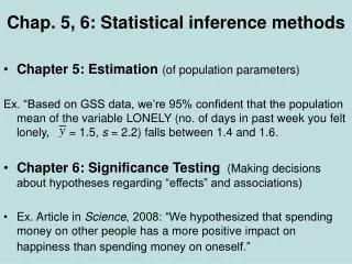
Using Simulation Methods to Introduce Statistical Inference
Using Simulation Methods to Introduce Statistical Inference. Patti Frazer Lock Kari Lock Morgan Cummings Professor of Mathematics Assistant Professor of the Practice St. Lawrence University Duke University AMATYC November, 2012. The Lock 5 Team. Robin & Patti St. Lawrence.

Using Simulation Methods to Introduce Statistical Inference
E N D
Presentation Transcript
Using Simulation Methods to Introduce Statistical Inference Patti Frazer Lock Kari Lock Morgan Cummings Professor of Mathematics Assistant Professor of the Practice St. Lawrence University Duke University AMATYC November, 2012
The Lock5 Team Robin & Patti St. Lawrence Dennis Iowa State Eric UNC/Duke Kari Harvard/Duke
New Simulation Methods “The Next Big Thing” United States Conference on Teaching Statistics, May 2011 Common Core State Standards in Mathematics Increasingly used in the disciplines
New Simulation Methods Increasingly important in DOING statistics Outstanding for use in TEACHING statistics Help students understand the key ideas of statistical inference
“New” Simulation Methods? "Actually, the statistician does not carry out this very simple and very tedious process, but his conclusions have no justification beyond the fact that they agree with those which could have been arrived at by this elementary method." -- Sir R. A. Fisher, 1936
Question Can you use your clicker? A. Yes B. No C. Not sure D. I don’t have a clicker
Question Do you teach Intro Stat? A. Very regularly (most semesters) B. Regularly (most years) C. Occasionally D. Rarely (every few years) E. Never (or not yet)
Question How familiar are you with simulation methods such as bootstrap confidence intervals and randomization tests? A. Very B. Somewhat C. A little D. Not at all E. Never heard of them before!
Bootstrap Confidence Intervals and Randomization Hypothesis Tests
First: Bootstrap Confidence Intervals
Example 1: What is the average price of a used Mustang car? Select a random sample of n=25 Mustangs from a website (autotrader.com) and record the price (in $1,000’s) for each car.
Sample of Mustangs: Our best estimate for the average price of used Mustangs is $15,980, but how accurate is that estimate?
Our best estimate for the average price of used Mustangs is $15,980, but how accurate is that estimate? We would like some kind of margin of error or a confidence interval. Key concept: How much can we expect the sample means to vary just by random chance?
Traditional Inference 1. Check conditions CI for a mean 2. Which formula? OR 3. Calculate summary stats , 4. Find t* 5. df? 95% CI df=251=24 t*=2.064 6. Plug and chug 7. Interpret in context
“We are 95% confident that the mean price of all used Mustang cars is between $11,390 and $20,570.” We arrive at a good answer, but the process is not very helpful at building understanding of the key ideas. In addition, our students are often great visual learners but get nervous about formulas and algebra. Can we find a way to use their visual intuition?
Brad Efron Stanford University “Let your data be your guide.” Bootstrapping Assume the “population” is many, many copies of the original sample.
Original Sample A simulated “population” to sample from
Brad Efron Stanford University “Let your data be your guide.” Bootstrapping Assume the “population” is many, many copies of the original sample. Key idea: To see how a statistic behaves, we take many samples with replacement from the original sample using the same n.
Bootstrap Sample: Sample with replacement from the original sample, using the same sample size. Original Sample Bootstrap Sample
Original Sample Bootstrap Sample
BootstrapSample Bootstrap Statistic BootstrapSample Bootstrap Statistic Original Sample Bootstrap Distribution • ● • ● • ● ● ● ● Sample Statistic BootstrapSample Bootstrap Statistic
We need technology! StatKey www.lock5stat.com
StatKey Standard Error
Using the Bootstrap Distribution to Get a Confidence Interval Chop 2.5% in each tail Keep 95% in middle Chop 2.5% in each tail We are 95% sure that the mean price for Mustangs is between $11,930 and $20,238
What yes/no question do you want to ask the sample of people in this audience? Do you have an ipad? Do you smoke? Do you have a smartphone? Do you exercise regularly? Did you vote republican?
What is your answer to the question? Yes No Example #2 : Find a 90% confidence interval for the proportion of people that attend AMATYC interested in introductory statistics who would answer “yes” to this question.
Why does the bootstrap work?
Sampling Distribution Population BUT, in practice we don’t see the “tree” or all of the “seeds” – we only have ONE seed µ
Bootstrap Distribution What can we do with just one seed? Bootstrap “Population” Estimate the distribution and variability (SE) of ’s from the bootstraps Grow a NEW tree! µ
Golden Rule of Bootstraps The bootstrap statistics are to the original statistic as the original statistic is to the population parameter.
Example 3: Diet Cola and Calcium What is the difference in mean amount of calcium excreted between people who drink diet cola and people who drink water? Find a 95% confidence interval for the difference in means.
Example 3: Diet Cola and Calcium www.lock5stat.com Statkey Select “CI for Difference in Means” Use the menu at the top left to find the correct dataset. Check out the sample: what are the sample sizes? Which group excretes more in the sample? Generate one bootstrap statistic. Compare it to the original. Generate a full bootstrap distribution (1000 or more). Use the “two-tailed” option to find a 95% confidence interval for the difference in means. What is your interval? Compare it with your neighbors. Is zero (no difference) in the interval? (If not, we can be confident that there is a difference.)
P-value: The probability of seeing results as extreme as, or more extreme than, the sample results, if the null hypothesis is true. Say what????
Example 1: Beer and Mosquitoes Does consuming beer attract mosquitoes? Experiment: 25 volunteers drank a liter of beer, 18 volunteers drank a liter of water Randomly assigned! Mosquitoes were caught in traps as they approached the volunteers.1 1Lefvre, T., et. al., “Beer Consumption Increases Human Attractiveness to Malaria Mosquitoes, ” PLoS ONE, 2010; 5(3): e9546.
Beer and Mosquitoes Number of Mosquitoes BeerWater 27 21 20 22 21 15 26 12 27 21 31 16 24 19 19 15 23 24 24 19 28 23 19 13 24 22 29 20 20 24 17 18 31 20 20 22 25 28 21 27 21 18 20 Does drinking beer actually attract mosquitoes, or is the difference just due to random chance? Beer mean = 23.6 Water mean = 19.22 Beer mean – Water mean = 4.38
Traditional Inference 1. Check conditions 2. Which formula? 5. Which theoretical distribution? 6. df? 7. find p-value 3. Calculate numbers and plug into formula 4. Plug into calculator 0.0005 < p-value < 0.001
Simulation Approach Number of Mosquitoes BeerWater 27 21 20 22 21 15 26 12 27 21 31 16 24 19 19 15 23 24 24 19 28 23 19 13 24 22 29 20 20 24 17 18 31 20 20 22 25 28 21 27 21 18 20 Does drinking beer actually attract mosquitoes, or is the difference just due to random chance? Beer mean = 23.6 Water mean = 19.22 Beer mean – Water mean = 4.38
Simulation Approach Number of Mosquitoes BeerWater 27 21 20 22 21 15 26 12 27 21 31 16 24 19 19 15 23 24 24 19 28 23 19 13 24 22 29 20 20 24 17 18 31 20 20 22 25 28 21 27 21 18 20 Find out how extreme these results would be, if there were no difference between beer and water. What kinds of results would we see, just by random chance?
Simulation Approach Number of Mosquitoes BeerWater 27 21 20 22 21 15 26 12 27 21 31 16 24 19 19 15 23 24 24 19 28 23 19 13 24 22 29 20 20 24 17 18 31 20 20 22 25 28 21 27 21 18 20 Number of Mosquitoes Beverage 27 21 20 22 21 15 26 12 27 21 31 16 24 19 19 15 23 24 24 19 28 23 19 13 24 22 29 20 20 24 17 18 31 20 20 22 25 28 21 27 21 18 20 Find out how extreme these results would be, if there were no difference between beer and water. What kinds of results would we see, just by random chance?
Simulation Approach BeerWater Number of Mosquitoes Beverage 20 22 21 15 26 12 27 21 31 16 24 19 19 15 23 24 24 19 28 23 19 13 24 22 29 20 20 24 17 18 31 20 20 22 25 28 21 27 21 18 20 Find out how extreme these results would be, if there were no difference between beer and water. What kinds of results would we see, just by random chance? 27 21 21 27 24 19 23 24 31 13 18 24 25 21 18 12 19 18 28 22 19 27 20 23 22 20 26 31 19 23 15 22 12 24 29 20 27 29 17 25 20 28
StatKey! www.lock5stat.com P-value
Traditional Inference 1. Which formula? 4. Which theoretical distribution? 5. df? 6. find p-value 2. Calculate numbers and plug into formula 3. Plug into calculator 0.0005 < p-value < 0.001
Beer and Mosquitoes • The Conclusion! The results seen in the experiment are very unlikely to happen just by random chance (just 1 out of 1000!) We have strong evidence that drinking beer does attract mosquitoes!
“Randomization” Samples Key idea: Generate samples that are based on the original sample AND consistent with some null hypothesis.
Example 2: Malevolent Uniforms Do sports teams with more “malevolent” uniforms get penalized more often?
Example 2: Malevolent Uniforms Sample Correlation = 0.43 Do teams with more malevolent uniforms commit more penalties, or is the relationship just due to random chance?
Simulation Approach Sample Correlation = 0.43 Find out how extreme this correlation would be, if there is no relationship between uniform malevolence and penalties. What kinds of results would we see, just by random chance?
Randomization by Scrambling Original sample Scrambled sample

