Statistical inference
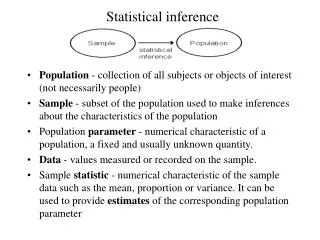
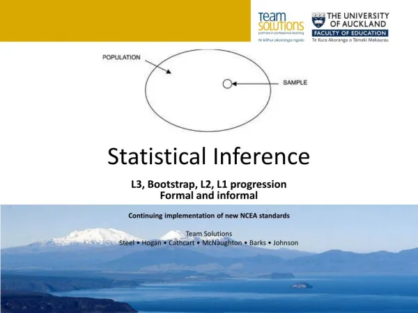
Statistical inference. Population - collection of all subjects or objects of interest (not necessarily people) Sample - subset of the population used to make inferences about the characteristics of the population

Statistical inference
E N D
Presentation Transcript
Statistical inference • Population - collection of all subjects or objects of interest (not necessarily people) • Sample - subset of the population used to make inferences about the characteristics of the population • Population parameter - numerical characteristic of a population, a fixed and usually unknown quantity. • Data - values measured or recorded on the sample. • Sample statistic - numerical characteristic of the sample data such as the mean, proportion or variance. It can be used to provide estimates of the corresponding population parameter
POINT AND INTERVAL ESTIMATION • Both types of estimates are needed for a given problem • Point estimate: Single value guess for parameter e.g. 1. For quantitative variables, the sample mean provides a point estimate of the unknown population mean 2. For binomial, the sample proportion is a point estimate of the unknown population proportion p. • Confidence interval: an interval that contains the true population parameter a high percentage (usually 95%) of the time • e.g. X= height of adult males in Ireland, • = avg. height of all adult males in Ireland • Point estimate: 5’10” 95 % C.I. : (5’ 8”, 6’0”)
Bias • The sampling distribution determines the expected value and variance of the sampling statistic. • Bias = distance between parameter and expected value of sample statistic. • If bias = 0, then the estimator is unbiased • Sample statistics can be classified as shown in the following diagrams. Low bias -high variability
When can bias occur ? • If the sample is not representative of the population being studied. • To minimise bias, sample should be chosen by random sampling, from a list of all individuals (sampling frame) • e.g. Sky News asks: Do British people support lower fuel prices ? Call 1-800-******* to register your opinion ? • Is this a random sample ? • In remainder of the course, we assume the samples are all random and representative of the population, hence the problem of bias goes away. Not always true in reality.
Convergence of probability • Recall Kerrich's coin tossing experiment- In 10,000 tosses of a coin you'd expect the number of heads (#heads) to approximately equal the number of tails • so #heads ½ #tosses • (#heads - ½ #tosses) can become large in absolute terms as the number of tosses increases (Fig 1). • in relative terms ( % of heads - 50%) -> 0 (Fig 2).
Law of Averages • as #tosses increases, you can think of this as #heads = ½ #tosses + chance error where chance error becomes large in absolute terms but small as % of #tosses as #tosses increases. • The Law of Averages states that an average result for n independent trials converges to a limit as n increases. • The law of averages does not work by compensation. A run of heads is just as likely to be followed by a head as by a tail because the outcomes of successive tosses are independent events
Law of Large Numbers • If X1,X2,….,Xnare independent random variables all with the same probability distribution with expected value µ and variance s2 then • is very likely to become very close to µ as n becomes very large. • Coin tossing is a simple example. • Law of large numbers says that: • But how close is it really ?
Sampling from exponential Draw a sample m=1 s2=1 0.217 1.372 0.125 0.030 0.221 0.430 0.986 0.131 1.345 0.606 0.889 0.113 1.026 1.874 3.042 ……………………… ……… • > mean(popsamp) • [1] 0.9809146 • > var(popsamp) • [1] 0.9953904
Samples of size 2 Population 0.217 1.372 0.125 0.030 0.221 0.430 0.986 0.131 1.345 0.606 0.889 0.113 1.026 1.874 3.042 ……………………… ……… • > mean(mss2) • [1] 0.9809146 • > var(mss2) • [1] 0.4894388 Sample 1: 0.217 1.372 Sample 2: 0.125 0.030 Sample 3: 0.217 0.889 …………………….
Samples of size 5 0.217 1.372 0.125 0.030 0.221 0.430 0.986 0.131 1.345 0.606 0.889 0.113 1.026 1.874 3.042 ……………………… ……… Sample 1: 0.217 1.372 0.125 0.030 0.221 Sample 2: 0.217 1.372 0.131 1.345 0.606 Sample 3: 0.889 0.113 1.026 1.874 3.042 ……………………. • > mean(mss5) • [1] 0.9809146 • > var(mss5) • [1] 0.201345
Sampling Distributions • Different samples give different values for sample statistics. By taking many different samples and calculating a sample statistic for each sample (e.g. the sample mean), you could then draw a histogram of all the sample means. A statistic from a sample or randomised experiment can be regarded as a random variable and the histogram is an approximation to its probability distribution. The term sampling distribution is used to describe this distribution, i.e. how the statistic (regarded as a random variable) varies if random samples are repeatedly taken from the population. • If the sampling distribution is known then the ability of the sample statistic to estimate the corresponding population parameter can be determined.
From the sample we can calculate Sampling Distribution of the Sample Mean • Usually both µ and are unknown, and we want primarily to estimate µ. • The sample mean is an estimate of µ, but how accurate ? • Sampling distribution depends on sample size n:
Sampling distribution of sample mean Sample mean is unbiased
Central Limit Theorem • The Central Limit Theorem says that the sample mean is approximately Normally distributed even if the original measurements were not Normally distributed. regardless of the shape of the probability distributions of X1, X2, ... .
Properties of sample mean • The sample mean is always unbiased • As n increases, the distribution becomes narrower - that is, the sample means cluster more tightly around µ. In fact the variance is inversely proportional to n • The square root of this variance, is called the "standard error" of This gives accuracy of the sample mean
Generating a sampling distribution • Step 1: Collect samples of size n (=5) from distribution F: xsample_rnorm(5000) xsample_matrix(xsample,ncol=5) > xsample[1,] [1] -0.9177649 -1.3931840 -1.6566304 -0.6219027 -1.834399 xsample[10,] [1] 0.3239556 -0.3127396 -1.3713074 0.9812672 -0.918144 • Step 2: Compute sample statistic for( i in 1:1000){samplemean[i]_mean(sample[i,])} > samplemeans[1] [1] -1.284776 • Step 3: Compute histogram of sample statistics hist(samplemean)
Sampling distribution of s2 • What is it’s sampling distribution ? • Sums of squares of i.i.d normals are chi-squared with as many d.f. as there are terms.

