Statistical Inference
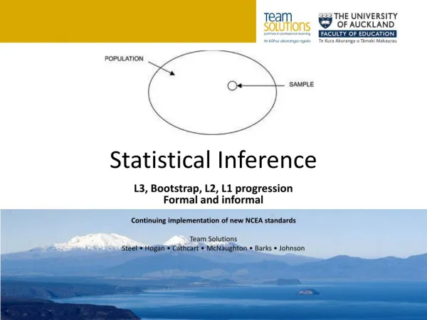
Statistical Inference. Using our sample to infer about our population. What is going on in the sample is of little actual interest to us – we are only interested in what it can tell us about the population. That is, we want to generalize about the population using the data from our sample.

Statistical Inference
E N D
Presentation Transcript
Statistical Inference Using our sample to infer about our population. What is going on in the sample is of little actual interest to us – we are only interested in what it can tell us about the population. That is, we want to generalize about the population using the data from our sample. Example: we don’t care what 1,000 randomly chosen Americans think about politics, we care about what these 1,000 Americans indicate about the overall population. To do this, we’ll learn inferential statistics.
Sampling Error It is possible that we follow all of the correct procedures to get a representative sample but we still don’t get one – this is called Sampling Error. We can randomly choose voters and the first 1,000 turn out to be Republicans. - so we must always account for the possibility that our sample isn’t really representative. That is why inferential statistics are always uncertain. We will learn how to quantify that uncertainty and thereby say how possible it is that we are wrong due to a poor sample.
What does it mean when we find a relationship in our sample? It can mean very little. It would be very hard to find absolutely no relationship in our sample. For example, there is no reason to believe that in the general population there is a relationship between height and party identification. So if there is no relationship in the population and if 40% of the population are Republicans, 38% are Democrats and 22% are Independents, what would I need to find in my sample so that there was no relationship in the sample? That for each height there is exactly a 40-38-22 split.
That is, Among tall people we would see a 40-38-22 split, and among medium people and short people the same split. Or the following: Short Medium Tall Republican 40% 40% 40% Indep. 22% 22% 22% Democrat 38% 38% 38% 100% 100% 100% Because there is the same breakdown for Party ID for every height category, we see no relationship between the two variables.
Is this what we need to see to conclude that there is no relationship in the population? No. What if we saw: Short Medium Tall Republican 42% 40% 38% Indep. 22% 22% 22% Democrat 36% 38% 40% 100% 100% 100% Here there is a (very slight) relationship in the sample between height and party identification. But is it strong enough to conclude that such a relationship exists in the population? Unless the sample is very big, no, its more likely that just by chance we chose a couple of extra tall Democrats. Changing our sample a little bit (or giving a couple people in our sample lifts in their shoes) could erase this relationship or push it into the other direction. So we need to see a relationship in our sample that is strong enough to conclude that a similar relationship exists in our population. The stronger the relationship in the sample is, the more confident we will be in concluding that such a relationship exists in the population as well.
Steps of Hypothesis Testing 1. State Research Hypothesis: HR & Null Hypothesis: H0 Choose p (probability) value – most likely .05 • Weight chance of Type I error vs. Type II 2. Choose appropriate test. 3. Compute test statistic. 4. Get critical value. 5. Compare test statistic with critical value. 6.7., 8. Make your Conclusion with a probability level. If test statistic > critical value “Reject the null hypothesis and temporarily accept the research hypothesis at the (.__) level.” .__ is given by p If test statistic < critical value…. “Fail to reject the null hypothesis at the (.__) level”
Think about hypothesis testing and significance tests in terms of a smoke detector Type I error – alarm without a fire Type II error – fire without an alarm.
No Fire Fire No Alarm Alarm “Alarm” means you think you’ve found something. “Fire” means there is something to find.
TRUE STATE H0 HA Accept H0 Reject H0
Pr(Rejecting H0 | H0) = Pr(Type I error | H0) = α α is the probability level we choose at step 1 of hypothesis testing 1- α measures our confidence that any alarm bells we hear are genuine. High confidence means rarely setting off false alarms.

