Statistical Inference
Statistical Inference. Dr. Mona Hassan Ahmed Prof. of Biostatistics HIPH, Alexandria University. Lesson Objectives. Know what is Inference Know what is parameter estimation Understand hypothesis testing & the “types of errors” in decision making. Know what the a -level means.


Statistical Inference
E N D
Presentation Transcript
Statistical Inference Dr. Mona Hassan Ahmed Prof. of Biostatistics HIPH, Alexandria University
Lesson Objectives • Know what is Inference • Know what is parameter estimation • Understand hypothesis testing & the “types of errors” in decision making. • Know what the a-level means. • Learn how to use test statistics to examine hypothesis about population mean, proportion
Inference Use a random sample to learn something about a larger population
Inference • Two ways to make inference • Estimation of parameters * Point Estimation (X or p) * Intervals Estimation • Hypothesis Testing
X Statistic Parameter ____ estimates Mean: Standard deviation: s ____ estimates p ____ estimates Proportion: from sample from entire population
Estimation of parameters Population Point estimate Interval estimate I am 95% confident that is between 40 & 60 Mean X = 50 Mean, , is unknown Sample
Parameter = Statistic ± Its Error
Sampling Distribution X or P X or P X or P
Standard Error Quantitative Variable Qualitative Variable
Confidence Interval α/2 α/2 1 - α _ X Z-axis SE SE 95% Samples X - 1.96 SE X + 1.96 SE
Confidence Interval α/2 α/2 1 - α p Z-axis SE SE 95% Samples p + 1.96 SE p - 1.96 SE
Example (Sample size≥30) An epidemiologist studied the blood glucose level of a random sample of 100 patients. The mean was 170, with a SD of 10. SE= 10/10 = 1 Then CI: = 170 + 1.96 1 168.04 ≥ 171.96 = X + Z SE 95%
Example (Proportion) In a survey of 140 asthmatics, 35% had allergy to house dust. Construct the 95% CI for the population proportion. = p + Z 0.35 – 1.96 0.04 ≥ 0.35 + 1.96 0.04 0.27 ≥ 0.43 27% ≥ 43% In a survey of 140 asthmatics, 35% had allergy to house dust. Construct the 95% CI for the population proportion. = p + Z 0.35 – 1.96 0.04 ≥ 0.35 + 1.96 0.04 0.27 ≥ 0.43 27% ≥ 43% P(1-p) 0.35(1-0.35) SE = = 0.04 n 140
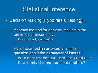
Hypothesis testing A statistical method that uses sample data to evaluate a hypothesis about a population parameter. It is intended to help researchers differentiate between real and random patterns in the data.
What is a Hypothesis? An assumption about the population parameter. I assume the mean SBP of participants is 120 mmHg
Null & Alternative Hypotheses • H0Null Hypothesisstates the Assumption to be tested e.g. SBP of participants = 120 (H0: m = 120). • H1 Alternative Hypothesis is the opposite of the null hypothesis (SBP of participants ≠ 120(H1: m≠ 120). Itmay or may not be accepted and it is the hypothesis that is believed to be true by the researcher
Level of Significance,a • Defines unlikely values of sample statistic if null hypothesis is true. Called rejection region of sampling distribution • Typical values are 0.01, 0.05 • Selected by the Researcher at the Start • Provides the Critical Value(s) of the Test
Level of Significance,aand the Rejection Region Critical Value(s) a Rejection Regions 0
Result Possibilities H0: Innocent Hypothesis Test Jury Trial Actual Situation Actual Situation Innocent Guilty H True H False Verdict Decision 0 0 Accept Type II Correct Error Innocent 1 - a H b ) Error ( 0 Type I Reject Power Error Correct Guilty Error H (1 - ) b 0 ( ) a False Positive False Negative
β Factors Increasing Type II Error • True Value of Population Parameter • Increases When Difference Between Hypothesized Parameter & True Value Decreases • Significance Level a • Increases When a Decreases • Population Standard Deviation s • Increases When sIncreases • Sample Size n • Increases When n Decreases b d b a b s b n
p Value Test • Probability of Obtaining a Test Statistic More Extreme (£ or ³) than Actual Sample Value Given H0 Is True • Called Observed Level of Significance • Used to Make Rejection Decision • If p value ³ a, Do Not Reject H0 • If p value < a, Reject H0
State H0H0 :m = 120 State H1H1 : m 120 Choose aa = 0.05 Choose n n = 100 Choose Test:Z, t, X2 Test (or p Value) Hypothesis Testing: Steps Test the Assumption that the true mean SBP of participants is 120 mmHg.
Compute Test Statistic (or compute P value) Search for Critical Value Make Statistical Decision rule Express Decision Hypothesis Testing: Steps
One sample-mean Test • Assumptions • Population isnormally distributed • t test statistic
Example Normal Body Temperature What is normal body temperature? Is it actually 37.6oC (on average)? State the null and alternative hypotheses H0: m = 37.6oC Ha: m37.6oC
Example Normal Body Temp (cont) Data: random sample of n = 18 normal body temps 37.2 36.8 38.0 37.6 37.2 36.8 37.4 38.7 37.236.4 36.6 37.4 37.0 38.2 37.6 36.1 36.2 37.5 Summarize data with a test statistic Variable n Mean SD SE t PTemperature 18 37.22 0.68 0.161 2.38 0.029
Example Normal Body Temp (cont) Find the p-value Df = n – 1 = 18 – 1 = 17 From SPSS:p-value = 0.029 From t Table:p-value is between 0.05 and 0.01. Area to left of t = -2.11 equals area to right of t = +2.11. The value t = 2.38 is between column headings 2.110& 2.898 in table, and for df =17, the p-values are 0.05 and 0.01. t -2.11 +2.11
Example Normal Body Temp (cont) Decide whether or not the result is statistically significant based on the p-value Using a = 0.05 as the level of significance criterion, the results are statistically significant because 0.029 is less than 0.05. In other words, we can reject the null hypothesis. Report the Conclusion We can conclude, based on these data, that the mean temperature in the human population does not equal 37.6.
One-sample test for proportion • Involves categorical variables • Fraction or % of population in a category • Sample proportion (p) • Test is called Z test where: • Z is computed value • πis proportion in population (null hypothesis value) Critical Values: 1.96 at α=0.05 2.58 at α=0.01
Example • In a survey of diabetics in a large city, it was found that 100 out of 400 have diabetic foot. Can we conclude that 20 percent of diabetics in the sampled population have diabetic foot. • Test at the a =0.05 significance level.
Solution Ho: π = 0.20 H1: π 0.20 = 2.50 Critical Value: 1.96 Decision: Reject Reject We have sufficient evidence to reject the Ho value of 20% We conclude that in the population of diabetic the proportion who have diabetic foot does not equal 0.20 .025 .025 -1.96 +1.96 0 Z