Statistical Inference
Statistical Inference. The larger the sample size (n) the more confident you can be that your sample mean is a good representation of the population mean. In other words, the "n" justifies the means. ~ Ancient Kung Foole Proverb. One- and Two Tailed Probabilities. One-tailed

Statistical Inference
E N D
Presentation Transcript
The larger the sample size (n) the more confident you can be that your sample mean is a good representation of the population mean. In other words, the "n" justifies the means. ~ Ancient Kung Foole Proverb
One- and Two Tailed Probabilities • One-tailed • The probability that an observation will occur at one end of the sampling distribution. • Two-tailed • The probability that an observation will occur at either extreme of the sampling distribution.
Hypothesis Testing • Conceptual (Research) Hypothesis • A general statement about the relationship between the independent and dependent variables • Statistical Hypothesis • A statement that can be shown to be supported or not supported by the data.
Statistical Significance Testing • Indirect Proof of a Hypothesis • Modus Tollens • A procedure of falsification that relies on a single observation. • Null Hypothesis • A statement that specifies no relationship or difference on a population parameter. • Alternative Hypothesis • A statement that specifies some value other than the null hypothesis is true.
Rejecting the Null • Alpha Level • The level of significant set by the experimenter. It is the confidence with which the researcher can decide to reject the null hypothesis. • Significance Level • The probability value used to conclude that the null hypothesis is an incorrect statement. Common significance levels are .05, .01 and .001.
Two Types of Error • Type I • When a researcher rejects the null hypothesis when in fact it is true. The probability of a type I error is α. • Type II • An error that occurs when a researcher fails to reject a null hypothesis that should be rejected. The probability of a Type II error is β.
Type 1 Error & Type 2 Error Scientist’s Decision Reject null hypothesis Fail to reject null hypothesis Type 1 Error Correct Decision probability = Probability = 1- Correct decision Type 2 Error probability = 1 - probability = Null hypothesis is true Null hypothesis is false Type 1 Error = Type 2 Error = Cases in which you reject null hypothesis when it is really true Cases in which you fail to reject null hypothesis when it is false
The OJ Trial For a nice tutorial go to: http://www.socialresearchmethods.net/OJtrial/ojhome.htm
One sample z-test • Used when we know µ and σ. • Generalization of calculating the probability of a score. • We are now calculating the probability of a sample given µ and σ.
The Problems with SST • We misunderstand what it does tell us. • It does not tell us what we want to know. • We often overemphasize SST.
Four Important Questions • Is there a real relationship in the population? Statistical Significance • How large is the relationship? Effect Size or Magnitude • Is it a relationship that has important, powerful, useful, meaningful implications? Practical Significance • Why is the relationship there? ??????
SST is all about . . . • Sampling Error • The difference between what I see in my sample and what exists in the target population. • Simply because I sampled, I could be wrong. • This is a threat to Internal Validity
How it works: • Assume sampling error occurred; there is no relationship in the population. • Build a statistical scenario based on this null hypothesis • How likely is it I got the sample value I got when the null hypothesis is true? (This is the fabled p-value.)
How it works (cont’d): • How unlikely does my result have to be to rule out sampling error? alpha (). • If p< , then our result is statistically rare, is unlikely to occur when there isn’t a relationship in the population.
What it does tell us • What is the probability that we would see a relationship in our sample when there is no relationship in the population? • Can we rule out sampling error as a competing hypothesis for our finding?
What it does not tell us • Whether the null hypothesis is true. • Whether our results will replicate. • Whether our research hypothesis is true. • How big the effect or relationship is. • How important the results are. • Why there is a relationship.
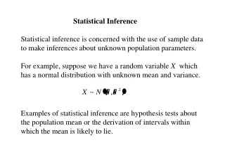
From Z to t… • In a Z test, you compare your sample to a known population, with a known mean and standard deviation. • In real research practice, you often compare two or more groups of scores to each other, without any direct information about populations. • Nothing is known about the populations that the samples are supposed to come from.
The t Test for a Single Sample • The single sample t test is used to compare a single sample to a population with a known mean but an unknown variance. • The formula for the t statistic is similar in structure to the Z, except that the t statistic uses estimated standard error.
From Z to t… Note lowercase “s”.
Degrees of Freedom • The number you divide by (the number of scores minus 1) to get the estimated population variance is called the degrees of freedom. • The degrees of freedom is the number of scores in a sample that are “free to vary”.
Degrees of Freedom • Imagine a very simple situation in which the individual scores that make up a distribution are 3, 4, 5, 6, and 7. • If you are asked to tell what the first score is without having seen it, the best you could do is a wild guess, because the first score could be any number. • If you are told the first score (3) and then asked to give the second, it too could be any number.
Degrees of Freedom • The same is true of the third and fourth scores – each of them has complete “freedom” to vary. • But if you know those first four scores (3, 4, 5, and 6) and you know the mean of the distribution (5), then the last score can only be 7. • If, instead of the mean and 3, 4, 5, and 6, you were given the mean and 3, 5, 6, and 7, the missing score could only be 4.
The t Distribution • In the Z test, you learned that when the population distribution follows a normal curve, the shape of the distribution of means will also be a normal curve. • However, this changes when you do hypothesis testing with an estimated population variance. • Since our estimate of is based on our sample… • And from sample to sample, our estimate of will change, or vary… • There is variation in our estimate of , and more variation in the t distribution.
The t Distribution • Just how much the t distribution differs from the normal curve depends on the degrees of freedom. • The t distribution differs most from the normal curve when the degrees of freedom are low (because the estimate of the population variance is based on a very small sample). • Most notably, when degrees of freedom is small, extremely large t ratios (either positive or negative) make up a larger-than-normal part of the distribution of samples.
The t Distribution • This slight difference in shape affects how extreme a score you need to reject the null hypothesis. • As always, to reject the null hypothesis, your sample mean has to be in an extreme section of the comparison distribution of means.
The t Distribution • However, if the distribution has more of its means in the tails than a normal curve would have, then the point where the rejection region begins has to be further out on the comparison distribution. • Thus, it takes a slightly more extreme sample mean to get a significant result when using a t distribution than when using a normal curve.
The t Distribution • For example, using the normal curve, 1.96 is the cut-off for a two-tailed test at the .05 level of significance. • On a t distribution with 3 degrees of freedom (a sample size of 4), the cutoff is 3.18 for a two-tailed test at the .05 level of significance. • If your estimate is based on a larger sample of 7, the cutoff is 2.45, a critical score closer to that for the normal curve.
The t Distribution • If your sample size is infinite, the t distribution is the same as the normal curve.
Since it takes into account the changing shape of the distribution as n increases, there is a separate curve for each sample size (or degrees of freedom). However, there is not enough space in the table to put all of the different probabilities corresponding to each possible t score. The t table lists commonly used critical regions (at popular alpha levels).
If your study has degrees of freedom that do not appear on the table, use the next smallest number of degrees of freedom. Just as in the normal curve table, the table makes no distinction between negative and positive values of t because the area falling above a given positive value of t is the same as the area falling below the same negative value.
The t Test for a Single Sample: Example You are a chicken farmer… if only you had paid more attention in school. Anyhow, you think that a new type of organic feed may lead to plumper chickens. As every chicken farmer knows, a fat chicken sells for more than a thin chicken, so you are excited. You know that a chicken on standard feed weighs, on average, 3 pounds. You feed a sample of 25 chickens the organic feed for several weeks. The average weight of a chicken on the new feed is 3.49 pounds with a standard deviation of 0.90 pounds. Should you switch to the organic feed? Use the .05 level of significance.
Hypothesis Testing • State the research question. • State the statistical hypothesis. • Set decision rule. • Calculate the test statistic. • Decide if result is significant. • Interpret result as it relates to your research question.
The t Test for a Single Sample: Example • State the research question. • Does organic feed lead to plumper chickens? • State the statistical hypothesis.
The t Test for a Single Sample: Example • Calculate the test statistic.
The t Test for a Single Sample: Example • Decide if result is significant. • Reject H0, 2.72 > 1.711 • Interpret result as it relates to your research question. • The chickens on the organic feed weigh significantly more than the chickens on the standard feed.