Ensembles for Cost-Sensitive Learning
Ensembles for Cost-Sensitive Learning. Thomas G. Dietterich Department of Computer Science Oregon State University Corvallis, Oregon 97331 http://www.cs.orst.edu/~tgd. Outline. Cost-Sensitive Learning Problem Statement; Main Approaches Preliminaries Standard Form for Cost Matrices

Ensembles for Cost-Sensitive Learning
E N D
Presentation Transcript
Ensembles for Cost-Sensitive Learning Thomas G. Dietterich Department of Computer Science Oregon State University Corvallis, Oregon 97331 http://www.cs.orst.edu/~tgd
Outline • Cost-Sensitive Learning • Problem Statement; Main Approaches • Preliminaries • Standard Form for Cost Matrices • Evaluating CSL Methods • Costs known at learning time • Costs unknown at learning time • Open Problems
Cost-Sensitive Learning • Learning to minimize the expected cost of misclassifications • Most classification learning algorithms attempt to minimize the expected number of misclassification errors • In many applications, different kinds of classification errors have different costs, so we need cost-sensitive methods
Examples of Applications with Unequal Misclassification Costs • Medical Diagnosis: • Cost of false positive error: Unnecessary treatment; unnecessary worry • Cost of false negative error: Postponed treatment or failure to treat; death or injury • Fraud Detection: • False positive: resources wasted investigating non-fraud • False negative: failure to detect fraud could be very expensive
Related Problems • Imbalanced classes: Often the most expensive class (e.g., cancerous cells) is rarer and more expensive than the less expensive class • Need statistical tests for comparing expected costs of different classifiers and learning algorithms
Example Misclassification Costs Diagnosis of Appendicitis • Cost Matrix: C(i,j) = cost of predicting class i when the true class is j
Estimating Expected Misclassification Cost • Let M be the confusion matrix for a classifier: M(i,j) is the number of test examples that are predicted to be in class i when their true class is j
Estimating Expected Misclassification Cost (2) • The expected misclassification cost is the Hadamard product of M and C divided by the number of test examples N: Si,j M(i,j) * C(i,j) / N • We can also write the probabilistic confusion matrix: P(i,j) = M(i,j) / N. The expected cost is then P * C
Interlude:Normal Form for Cost Matrices • Any cost matrix C can be transformed to an equivalent matrix C’ with zeroes along the diagonal • Let L(h,C) be the expected loss of classifier h measured on loss matrix C. • Defn: Let h1 and h2 be two classifiers. C and C’ are equivalent if L(h1,C) > L(h2,C) iff L(h1,C’) > L(h2,C’)
Theorem(Margineantu, 2001) • Let D be a matrix of the form • If C2 = C1 + D, then C1 is equivalent to C2
Proof • Let P1(i,k) be the probabilistic confusion matrix of classifier h1, and P2(i,k) be the probabilistic confusion matrix of classifier h2 • L(h1,C) = P1 * C • L(h2,C) = P2 * C • L(h1,C) – L(h2,C) = [P1 – P2] * C
Proof (2) • Similarly, L(h1,C’) – L(h2, C’) = [P1 – P2] * C’ = [P1 – P2] * [C + D] = [P1 – P2] * C + [P1 – P2] * D • We now show that [P1 – P2] * D = 0, from which we can conclude that L(h1,C) – L(h2,C) = L(h1,C’) – L(h2,C’) and hence, C is equivalent to C’.
Proof (3) [P1 – P2] * D = SiSk [P1(i,k) – P2(i,k)] * D(i,k) = SiSk [P1(i,k) – P2(i,k)] * dk = Skdk Si [P1(i,k) – P2(i,k)] = Skdk Si [P1(i|k) P(k) – P2(i|k) P(k)] = Skdk P(k) Si [P1(i|k) – P2(i|k)] = Skdk P(k) [1 – 1] = 0
Proof (4) • Therefore, L(h1,C) – L(h2,C) = L(h1,C’) – L(h2,C’). • Hence, if we set dk = –C(k,k), then C’ will have zeroes on the diagonal
End of Interlude • From now on, we will assume that C(i,i) = 0
Interlude 2: Evaluating Cost-Sensitive Learning Algorithms • Evaluation for a particular C: • BCOST and BDELTACOST procedures • Evaluation for a range of possible C’s: • AUC: Area under the ROC curve • Average cost given some distribution D(C) over cost matrices
Two Statistical Questions • Given a classifier h, how can we estimate its expected misclassification cost? • Given two classifiers h1 and h2, how can we determine whether their misclassification costs are significantly different?
Estimating Misclassification Cost: BCOST • Simple Bootstrap Confidence Interval • Draw 1000 bootstrap replicates of the test data • Compute confusion matrix Mb, for each replicate • Compute expected cost cb = Mb * C • Sort cb’s, form confidence interval from the middle 950 points (i.e., from c(26) to c(975)).
Comparing Misclassification Costs: BDELTACOST • Construct 1000 bootstrap replicates of the test set • For each replicate b, compute the combined confusion matrix Mb(i,j,k) = # of examples classified as i by h1, as j by h2, whose true class is k. • Define D(i,j,k) = C(i,k) – C(j,k) to be the difference in cost when h1 predicts class i, h2 predicts j, and the true class is k. • Compute db = Mb * D • Sort the db’s and form a confidence interval [d(26), d(975)] • If this interval excludes 0, conclude that h1 and h2 have different expected costs
ROC Curves • Most learning algorithms and classifiers can tune the decision boundary • Probability threshold: P(y=1|x) > q • Classification threshold: f(x) > q • Input example weights l • Ratio of C(0,1)/C(1,0) for C-dependent algorithms
ROC Curve • For each setting of such parameters, given a validation set, we can compute the false positive rate: fpr = FP/(# negative examples) and the true positive rate tpr = TP/(# positive examples) and plot a point (tpr, fpr) • This sweeps out a curve: The ROC curve
AUC: The area under the ROC curve • AUC = Probability that two randomly chosen points x1 and x2 will be correctly ranked: P(y=1|x1) versus P(y=1|x2) • Measures correct ranking (e.g., ranking all positive examples above all negative examples) • Does not require correct estimates of P(y=1|x)
Direct Computation of AUC(Hand & Till, 2001) • Direct computation: • Let f(xi) be a scoring function • Sort the test examples according to f • Let r(xi) be the rank of xi in this sorted order • Let S1 = S{i: yi=1} r(xi) be the sum of ranks of the positive examples • AUC = [S1 – n1(n1+1)/2] / [n0 n1] where n0 = # negatives, n1 = # positives
Using the ROC Curve • Given a cost matrix C, we must choose a value for q that minimizes the expected cost • When we build the ROC curve, we can store q with each (tpr, fpr) pair • Given C, we evaluate the expected cost according to p0 * fpr * C(1,0) + p1 * (1 – tpr) * C(0,1) where p0 = probability of class 0, p1 = probability of class 1 • Find best (tpr, fpr) pair and use corresponding threshold q
End of Interlude 2 • Hand and Till show how to generalize the ROC curve to problems with multiple classes • They also provide a confidence interval for AUC
Outline • Cost-Sensitive Learning • Problem Statement; Main Approaches • Preliminaries • Standard Form for Cost Matrices • Evaluating CSL Methods • Costs known at learning time • Costs unknown at learning time • Variations and Open Problems
Two Learning Problems • Problem 1: C known at learning time • Problem 2: C not known at learning time (only becomes available at classification time) • Learned classifier should work well for a wide range of C’s
Learning with known C • Goal: Given a set of training examples {(xi, yi)} and a cost matrix C, • Find a classifier h that minimizes the expected misclassification cost on new data points (x*,y*)
Two Strategies • Modify the inputs to the learning algorithm to reflect C • Incorporate C into the learning algorithm
Strategy 1:Modifying the Inputs • If there are only 2 classes and the cost of a false positive error is l times larger than the cost of a false negative error, then we can put a weight of l on each negative training example • l = C(1,0) / C(0,1) • Then apply the learning algorithm as before
Some algorithms are insensitive to instance weights • Decision tree splitting criteria are fairly insensitive (Holte, 2000)
Setting l By Class Frequency • Set l/ 1/nk, where nk is the number of training examples belonging to class k • This equalizes the effective class frequencies • Less frequent classes tend to have higher misclassification cost
Setting l by Cross-validation • Better results are obtained by using cross-validation to set l to minimize the expected error on the validation set • The resulting l is usually more extreme than C(1,0)/C(0,1) • Margineantu applied Powell’s method to optimize lk for multi-class problems
Comparison Study Grey: CV l wins; Black: ClassFreq wins; White: tie 800 trials (8 cost models * 10 cost matrices * 10 splits)
Conclusions from Experiment • Setting l according to class frequency is cheaper gives the same results as setting l by cross validation • Possibly an artifact of our cost matrix generators
Strategy 2:Modifying the Algorithm • Cost-Sensitive Boosting • C can be incorporated directly into the error criterion when training neural networks (Kukar & Kononenko, 1998)
Cost-Sensitive Boosting(Ting, 2000) • Adaboost (“confidence weighted”) • Initialize wi = 1/N • Repeat • Fit ht to weighted training data • Compute et = Si yi ht(xi) wi • Set at = ½ * ln (1 + et)/(1 – et) • wi := wi * exp(–at yi ht(xi))/Zt • Classify using sign(Stat ht(x))
Three Variations • Training examples of the form (xi, yi, ci), where ci is the cost of misclassifying xi • AdaCost (Fan et al., 1998) • wi := wi * exp(–at yi ht(xi) bi)/Zt • bi = ½ * (1 + ci) if error = ½ * (1 – ci) otherwise • CSB2 (Ting, 2000) • wi := bi wi * exp(–at yi ht(xi))/Zt • bi = ci if error = 1 otherwise • SSTBoost (Merler et al., 2002) • wi := wi * exp(–at yi ht(xi) bi)/Zt • bi = ci if error • bi = 2 – ci otherwise • ci = w for positive examples; 1 – w for negative examples
Additional Changes • Initialize the weights by scaling the costs ci • wi = ci / Sj cj • Classify using “confidence weighting” • Let F(x) = Stat ht(x) be the result of boosting • Define G(x,k) = F(x) if k = 1 and –F(x) if k = –1 • predicted y = argminiSk G(x,k) C(i,k)
Experimental Results:(14 data sets; 3 cost ratios; Ting, 2000)
Open Question • CSB2, AdaCost, and SSTBoost were developed by making ad hoc changes to AdaBoost • Opportunity: Derive a cost-sensitive boosting algorithm using the ideas from LogitBoost (Friedman, Hastie, Tibshirani, 1998) or Gradient Boosting (Friedman, 2000) • Friedman’s MART includes the ability to specify C (but I don’t know how it works)
Outline • Cost-Sensitive Learning • Problem Statement; Main Approaches • Preliminaries • Standard Form for Cost Matrices • Evaluating CSL Methods • Costs known at learning time • Costs unknown at learning time • Variations and Open Problems
Learning with Unknown C • Goal: Construct a classifier h(x,C) that can accept the cost function at run time and minimize the expected cost of misclassification errors wrt C • Approaches: • Learning to estimate P(y|x) • Learn a “ranking function” such that f(x1) > f(x2) implies P(y=1|x1) > P(y=1|x2)
Learning Probability Estimators • Train h(x) to estimate P(y=1|x) • Given C, we can then apply the decision rule: • y’ = argminiSk P(y=k|x) C(i,k)
Good Class Probabilities from Decision Trees • Probability Estimation Trees • Bagged Probability Estimation Trees • Lazy Option Trees • Bagged Lazy Option Trees
Causes of Poor Decision Tree Probability Estimates • Estimates in leaves are based on a small number of examples (nearly pure) • Need to sub-divide “pure” regions to get more accurate probabilities
Probability Estimates are Extreme Single decision tree; 700 examples
P(y=1|x) 0.5 x Need to Subdivide “Pure” Leaves Consider a region of the feature space X. Suppose P(y=1|x) looks like this:
P(y=1|x) 0.5 x Probability Estimation versus Decision-making A simple CLASSIFIER will introduce one split predict class 1 predict class 0