Ensembles
Ensembles. An ensemble is a set of classifiers whose combined results give the final decision. test feature vector. classifier 1. classifier 2. classifier 3. super classifier. result. *. *A model is the learned decision rule . It can be as simple as a

Ensembles
E N D
Presentation Transcript
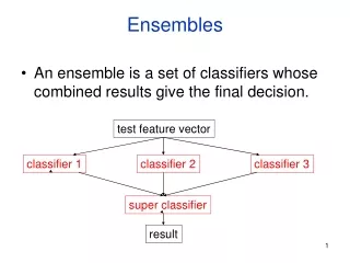
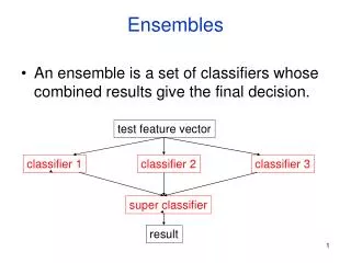
Ensembles • An ensemble is a set of classifiers whose combined results give the final decision. test feature vector classifier 1 classifier 2 classifier 3 super classifier result
* *A model is the learned decision rule. It can be as simple as a hyperplane in n-space (ie. a line in 2D or plane in 3D) or in the form of a decision tree or other modern classifier.
Boosting In More Detail(Pedro Domingos’ Algorithm) • Set all E weights to 1, and learn H1. • Repeat m times: increase the weights of misclassified Es, and learn H2,…Hm. • H1..Hm have “weighted majority” vote when classifying each test Weight(H)=accuracy of H on the training data
ADABoost • ADABoost booststhe accuracy of the original learning algorithm. • If the original learning algorithm does slightly better than 50% accuracy, ADABoost with a large enough number of classifiers is guaranteed to classify the training data perfectly.
ADABoost Weight Updating for j = 1 to N do /* go through training samples */ if h[m](xj) <> yj then error <- error + wj for j = 1 to N do if h[m](xj) = yj then w[j] <- w[j] * error/(1-error)
Sample Application: Insect Recognition Doroneuria (Dor) Using circular regions of interest selected by an interest operator, train a classifier to recognize the different classes of insects.
Boosting Comparison • ADTree classifier only(alternating decision tree) • Correctly Classified Instances 268 70.1571 % • Incorrectly Classified Instances 114 29.8429 % • Mean absolute error 0.3855 • Relative absolute error 77.2229 %
Boosting Comparison AdaboostM1 with ADTree classifier • Correctly Classified Instances 303 79.3194 % • Incorrectly Classified Instances 79 20.6806 % • Mean absolute error 0.2277 • Relative absolute error 45.6144 %
Boosting Comparison • RepTree classifier only(reduced error pruning) • Correctly Classified Instances 294 75.3846 % • Incorrectly Classified Instances 96 24.6154 % • Mean absolute error 0.3012 • Relative absolute error 60.606 %
Boosting Comparison • AdaboostM1 with RepTree classifier • Correctly Classified Instances 324 83.0769 % • Incorrectly Classified Instances 66 16.9231 % • Mean absolute error 0.1978 • Relative absolute error 39.7848 %
References • AdaboostM1: Yoav Freund and Robert E. Schapire (1996). "Experiments with a new boosting algorithm". Proc International Conference on Machine Learning, pages 148-156, Morgan Kaufmann, San Francisco. • ADTree: Freund, Y., Mason, L.: "The alternating decision tree learning algorithm". Proceeding of the Sixteenth International Conference on Machine Learning, Bled, Slovenia, (1999) 124-133.
Yu-Yu Chou’s Hierarchical Classifiers • Developed for pap smear analysis in which the categories were normal, abnormal(cancer), and artifact plus subclasses of each • More than 300 attributes per feature vector and little or no knowledge of what they were. • Large amount of training data making classifier construction slow or impossible.
Results • Our classifier was able to beat the handcrafted decision tree classifier that had taken Neopath years to develop. • It was tested successfully on another pap smear data set and a forest cover data set. • It was tested against bagging and boosting. It was better at detecting abnormal pap smears than both, and not as good at classifying normal ones as normal. It was slightly higher than both in overall classification rate.
Bayesian Learning • Bayes’ Rule provides a way to calculate probability of a hypothesis based on • its prior probability • the probability of observing the data, given that hypothesis • the observed data (feature vector)
Bayes’ Rule P(X | h) P(h) P(h | X) = ----------------- P(X) • h is the hypothesis (such as the class). • X is the feature vector to be classified. • P(X | h) is the prior probability that this feature vector occurs, given that h is true. • P(h) is the prior probability of hypothesis h. • P(X) = the prior probability of the feature vector X. • These priors are usually calculated from frequencies in the training data set. Often assumed constant and left out.
Example x1 x2 x3 y 0 0 0 1 0 0 1 0 0 1 0 1 0 1 1 1 1 0 0 0 1 0 1 1 1 1 0 0 1 1 1 0 • Suppose we want to know the probabilty of class 1 for feature vector [0,1,0]. • P(1 | [0,1,0]) = P([0,1,0] | 1) P(1) / P([0,1,0]) = (0.25) (0.5) / (.125) = 1.0 Of course the training set would be much bigger and for real data could include multiple instances of a given feature vector.
MAP • Suppose H is a set of candidate hypotheses. • We would like to find the most probable h in H. • hMAP is a MAP (maxiumum a posteriori) hypothesis if hMAP = argmax P(h | X) h H • This just says to calculate P(h | X) by Bayes’ rule for each possible class h and take the one that gets the highest score.
Cancer Test Example P(cancer) = .008 P(not cancer) = .992 P(positive | cancer) = .98 P(positive | not cancer) = .03 P(negative | cancer) = .02 P(negative | not cancer) =.97 Priors New patient’s test comes back positive. P(cancer | positive) = P(positive | cancer) P(cancer) = (.98) (.008) = .0078 P(not cancer | positive = P(positive | not cancer) P(not cancer) = (.03) (.992) = .0298 hMAP would say it’s not cancer. Depends strongly on priors!
Neural Net Learning • Motivated by studies of the brain. • A network of “artificial neurons” that learns a function. • Doesn’t have clear decision rules like decision trees, but highly successful in many different applications. (e.g. face detection) • Our hierarchical classifier used neural net classifiers as its components.