Ensembles
Explore boosting algorithms such as AdaBoost and comparison with classifiers like ADTree and RepTree. Learn about Neural Network Learning, Kernel Machines, and Support Vector Machines (SVM) for improved classification accuracy. Discover the concept of ensembles and the power of combining multiple classifiers.

Ensembles
E N D
Presentation Transcript
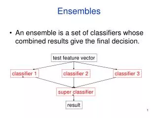
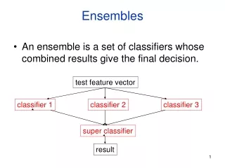
Ensembles • An ensemble is a set of classifiers whose combined results give the final decision. test feature vector classifier 1 classifier 2 classifier 3 super classifier result
* *A model is the learned decision rule. It can be as simple as a hyperplane in n-space (ie. a line in 2D or plane in 3D) or in the form of a decision tree or other modern classifier.
Boosting In More Detail(Pedro Domingos’ Algorithm) • Set all E weights to 1, and learn H1. • Repeat m times: increase the weights of misclassified Es, and learn H2,…Hm. • H1..Hm have “weighted majority” vote when classifying each test Weight(H)=accuracy of H on the training data
ADABoost • ADABoost booststhe accuracy of the original learning algorithm. • If the original learning algorithm does slightly better than 50% accuracy, ADABoost with a large enough number of classifiers is guaranteed to classify the training data perfectly.
ADABoost Weight Updating for j = 1 to N do /* go through training samples */ if h[m](xj) <> yj then error <- error + wj for j = 1 to N do if h[m](xj) = yj then w[j] <- w[j] * error/(1-error)
Sample Application: Insect Recognition Doroneuria (Dor) Using circular regions of interest selected by an interest operator, train a classifier to recognize the different classes of insects.
Boosting Comparison • ADTree classifier only(alternating decision tree) • Correctly Classified Instances 268 70.1571 % • Incorrectly Classified Instances 114 29.8429 % • Mean absolute error 0.3855 • Relative absolute error 77.2229 %
Boosting Comparison AdaboostM1 with ADTree classifier • Correctly Classified Instances 303 79.3194 % • Incorrectly Classified Instances 79 20.6806 % • Mean absolute error 0.2277 • Relative absolute error 45.6144 %
Boosting Comparison • RepTree classifier only(reduced error pruning) • Correctly Classified Instances 294 75.3846 % • Incorrectly Classified Instances 96 24.6154 % • Mean absolute error 0.3012 • Relative absolute error 60.606 %
Boosting Comparison AdaboostM1 with RepTree classifier • Correctly Classified Instances 324 83.0769 % • Incorrectly Classified Instances 66 16.9231 % • Mean absolute error 0.1978 • Relative absolute error 39.7848 %
References • AdaboostM1: Yoav Freund and Robert E. Schapire (1996). "Experiments with a new boosting algorithm". Proc International Conference on Machine Learning, pages 148-156, Morgan Kaufmann, San Francisco. • ADTree: Freund, Y., Mason, L.: "The alternating decision tree learning algorithm". Proceeding of the Sixteenth International Conference on Machine Learning, Bled, Slovenia, (1999) 124-133.
Neural Net Learning • Motivated by studies of the brain. • A network of “artificial neurons” that learns a function. • Doesn’t have clear decision rules like decision trees, but highly successful in many different applications. (e.g. face detection) • Our hierarchical classifier used neural net classifiers as its components.
Back-Propagation Illustration ARTIFICIAL NEURAL NETWORKS Colin Fahey's Guide (Book CD)
Kernel Machines • A relatively new learning methodology (1992) derived from statistical learning theory. • Became famous when it gave accuracy comparable to neural nets in a handwriting recognition class. • Was introduced to computer vision researchers by Tomaso Poggio at MIT who started using it for face detection and got better results than neural nets. • Has become very popular and widely used with packages available.
Support Vector Machines (SVM) • Support vector machines are learning algorithms that try to find a hyperplane that separates the different classes of data the most. • They are a specific kind of kernel machines based on two key ideas: • maximum margin hyperplanes • a kernel ‘trick’
Maximal Margin (2 class problem) In 2D space, a hyperplane is a line. In 3D space, it is a plane. margin hyperplane Find the hyperplane with maximal margin for all the points. This originates an optimization problem which has a unique solution.
Support Vectors • The weights i associated with data points are zero, except for those points closest to the separator. • The points with nonzero weights are called the support vectors (because they hold up the separating plane). • Because there are many fewer support vectors than total data points, the number of parameters defining the optimal separator is small.
Kernels • A kernel is just a similarity function. It takes 2 inputs and decides how similar they are. • Kernels offer an alternative to standard feature vectors. Instead of using a bunch of features, you define a single kernel to decide the similarity between two objects.
Kernels and SVMs • Under some conditions, every kernel function can be expressed as a dot product in a (possibly infinite dimensional) feature space (Mercer’s theorem) • SVM machine learning can be expressed in terms of dot products. • So SVM machines can use kernels instead of feature vectors.
The Kernel Trick The SVM algorithm implicitly maps the original data to a feature space of possibly infinite dimension in which data (which is not separable in the original space) becomes separable in the feature space. Feature space Rn Original space Rk 1 1 1 0 0 0 1 0 0 1 0 0 Kernel trick 1 0 0 0 1 1
Kernel Functions • The kernel function is designed by the developer of the SVM. • It is applied to pairs of input data to evaluate dot products in some corresponding feature space. • Kernels can be all sorts of functions including polynomials and exponentials.
Kernel Function used in our 3D Computer Vision Work • k(A,B) = exp(-2AB/2) • A and B are shape descriptors (big vectors). • is the angle between these vectors. • 2 is the “width” of the kernel.
What do SVMs solve? • The SVM is looking for the best separating plane in its alternate space. • It solves a quadratic programming optimization problem argmaxΣαj-1/2 Σαj αk yjyk(xj•xk) subject to αj > 0 and Σαjyj = 0. • The equation for the separator for these optimal αj is h(x) = sign(Σαjyj (x•xj) – b) α j j,k j j
Unsupervised Learning • Find patterns in the data. • Group the data into clusters. • Many clustering algorithms. • K means clustering • EM clustering • Graph-Theoretic Clustering • Clustering by Graph Cuts • etc
Clustering by K-means Algorithm Form K-means clusters from a set of n-dimensional feature vectors 1. Set ic (iteration count) to 1 2. Choose randomly a set of K means m1(1), …, mK(1). 3. For each vector xi, compute D(xi,mk(ic)), k=1,…K and assign xi to the cluster Cj with nearest mean. 4. Increment ic by 1, update the means to get m1(ic),…,mK(ic). 5. Repeat steps 3 and 4 until Ck(ic) = Ck(ic+1) for all k.
K-Means Classifier(shown on RGB color data) original data one RGB per pixel color clusters
For each cluster j K-Means EMThe clusters are usually Gaussian distributions. • Boot Step: • Initialize K clusters: C1, …, CK • Iteration Step: • Estimate the cluster of each datum • Re-estimate the cluster parameters (j,j) and P(Cj)for each cluster j. Expectation Maximization The resultant set of clusters is called a mixture model; if the distributions are Gaussian, it’s a Gaussian mixture.
EM Algorithm Summary • Boot Step: • Initialize K clusters: C1, …, CK • Iteration Step: • Expectation Step • Maximization Step (j,j) and p(Cj)for each cluster j.
EM Clustering using color and texture information at each pixel(from Blobworld)
Final Model for “trees” Initial Model for “trees” EM Final Model for “sky” Initial Model for “sky” EM for Classification of Images in Terms of their Color Regions
Sample Results cheetah