Download
1 / 16

E N D
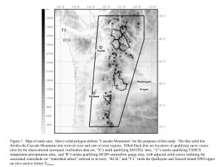
T.I. Seattle Washington Oregon Portland Figure 1. Map of study area. Heavy solid polygon defines “Cascade Mountains” for the purposes of this study. The thin solid line divides the Cascade Mountains into west-of-crest and east-of-crest regions. Filled black dots are locations of qualifying snow course sites for the observational snowpack verification data set, “X”s mark qualifying SNOTEL sites, “C”s marks qualifying USHCN temperature/precipitation sites, and “R”s marks qualifying HCDN streamflow gauge sites, with adjacent solid curves outlining the associated watersheds (or “watershed subset” referred to in text). “KUIL” and “T.I.” mark the Quillayute and Tatoosh Island NWS upper air sites used to define T850ons.
r = 0.94 – E0 = – 29.6% Figure 2. Scatter plot of annual runoff within the watershed subset (in percent of 1961-1990 mean) vs. west Cascade-averaged annual precipitation (also in percent of 1961-1990 mean). Also shown is best-fit line, correlation, and y-intercept.
(a) (b) (c) West of crest East of crest Figure 3. Example (for 1 April 2006) of information used to construct the snow course-based Cascade SWE volume used to verify the water-balance snowpack. (a) Total area covered by each 10-m elevation band (equivalent to the derivative with respect to height of the hypsometric curve) within the watershed subset shown in Fig. 1. Separate curves are shown for portions of the watersheds that are west and east of the crest, as defined by the polygons in Fig. 1. (b) Scatter plot of SWE depth vs. elevation, with linear fits, for stations west and east of the crest. (c) Estimate of SWE volume vs. elevation within the watershed subset, obtained by multiplying (a) x (b).
r = 0.95 1955-2007 trends in 1 Apr snowpack: Water Balance: -28% Snowcourse: -31% 0 Figure 4. Scatter plot of water-balance 1 April snowpack vs. snow-course 1 April snowpack, for years 1955-2007 (1955 was the first year of the snow-course snowpack time series). Values are in percent of 1961-1990 normal for SWE volume in the Cascade watershed subset. Also shown is the 1:1 line (thin dashed), the best-fit line (heavy dashed) with correlation, and the 1955-2007 trend values.
Water Balance SNOTEL Figure 5. Monthly snowpack derived from the water-balance model (solid) and from SNOTEL observations (dashed), expressed as a percent of the 1961-1990 normal 1 April SWE volume for the watershed subset, for water years 1992 through 2007. Water years are labeled at October 1 (the start of the water year).
1950-1997: -48% ± 34% (-10.3 ± 7.3 % dec-1) (a) 1930-2007: -23% ± 28% (-2.9 ± 3.6 % dec-1) 1976-2007: +19% ± 43% (+6.0 ± 13.7 % dec-1) Figure 6. (a) 1 April water-balance snowpack (% of 1961-1990 mean, thin solid curve); smoothed version (heavy solid curve); trend lines over the periods indicated (heavy dashed lines), with trend values (given in total percent change and percent per decade) and 95% confidence intervals listed. (b) As in (a), except for October-March west Cascade-averaged precipitation (% of 1961-1990 mean). (c) As in (a), except for November-March west Cascade-averaged temperature anomaly (°C). (d) As in (a), except for November-March mean 850-hPa temperature anomaly (°C) at KUIL when 850-hPa flow is onshore. Temperature anomalies are with respect to the 1961-1990 mean. (b) 1950-1997: -12% ± 20% (-2.5 ± 4.3 % dec-1) 1930-2007: +2% ± 16% (+0.2 ± 2.0 % dec-1) 1976-2007: +11% ± 26% (+3.6 ± 8.5 % dec-1)
(c) 1930-2007: +0.7 °C± 0.7 °C (+0.09 ± 0.09 °C dec-1) 1976-2007: +0.5 °C± 1.0 °C (+0.15 ± 0.32 °C dec-1) 1950-1997: +0.7 °C± 0.8 °C (+0.15 ± 0.18 °C dec-1) (d) 1930-2007: +0.9 °C± 0.8 °C (+0.12 ± 0.11 °C dec-1) 1976-2007: -0.1 °C± 1.2 °C (-0.02 ± 0.39 °C dec-1) 1950-1997: +1.5 °C± 1.0 °C (+0.31 ± 0.22 °C dec-1) Figure 6 (cont.).
(a) r = 0.80 Figure 7. (a) Scatter plot of water-balance 1 April snowpack vs. October-March west Cascade-averaged precipitation (both as % of 1961-1990 mean). (b) Scatter plot of water-balance 1 April snowpack vs. November-March west Cascade-averaged temperature anomaly (°C). (c) Scatter plot of water-balance 1 April snowpack vs. November-March mean 850-hPa temperature anomaly (°C) at KUIL when 850-hPa flow is onshore.
(b) r = -0.44 (c) r = -0.68 Figure 7 (cont.).
150° E 1 2 1 2 3 (b) SLP′for high snow 3 (a) Correlation 1 1 2 2 3 3 (c) SLP for high snow (d) SLP for low snow Figure 8. (a) Map of the regression coefficient between the winter (November-March mean) sea-level pressure field over the north Pacific Ocean region and the Cascade 1 April snowpack (from the water-balance). Location of Cascade Range indicated by star. Numbered circles indicate the set of three points within the domain whose SLP explains more of the variance in snowpack than any other set of three points. Box shows averaging area for the North Pacific Index (NPI). (b) Composite of the winter SLP anomaly field (hPa, as a departure from the 1961-1990 mean) during the five years with highest Cascade Snow Circulation (CSC) index. (c) Composite of the total winter SLP field (hPa) during the five years of highest CSC index. (d) Composite of the total winter SLP field (hPa) during the five years of lowest CSC index.
(a) Figure 9. (a) Time series of November-March mean CSC index (hPa, thin black curve), smoothed version (heavy gray curve), and means of CSC index during PDO epoch periods (heavy black lines). (b) Scatter plot of 1 April snowpack (from the water-balance, in % of 1961-1990 mean) vs. November-March mean CSC index (hPa, black circles) with best-fit line (black dashed) and correlation. (c) As in Fig. 6a, except the snowpack time-series has had the CSC-correlated part removed.
(b) r = 0.84 (c) 1930-2007: -16% ± 15% (-2.0 ± 1.9 % dec-1) 1976-2007: -5% ± 24% (-1.6 ± 7.9 % dec-1) 1950-1997: -9% ± 19% (-1.9 ± 4.0 % dec-1) Figure 9 (cont.).
1930-2007: -5 ± 20 days (-0.6 ± 2.6 days dec-1) 1950-1997: -16 ± 23 days (-3.3 ± 5.0 days dec-1) 1976-2007: +18 ± 35 days (+5.8 ± 11.3 days dec-1) 90% Melt-out date Max snowpack date 1930-2007: -5 ± 15 days (-0.6 ± 1.9 days dec-1) 1950-1997: -23 ± 18 days (-4.9 ± 3.9 days dec-1) 1976-2007: +5 ± 24 days (+1.7 ± 7.8 days dec-1) Figure 10. As in Fig. 6a, except showing Julian date of maximum snowpack (lower curves and lines) and of 90% melt-out (upper curves and lines), based on the water-balance monthly snowpack record.
Figure 11. Changes in December-February mean surface air temperature (°C) during the period 1976 to 2007, based on linear trends. The plot was generated using the temperature trend mapping web page provided by the NASA Goddard Institute for Space Studies (http://data.giss.nasa.gov/gistemp/maps), which uses the surface temperature data set described by Hansen et al. (2001). The white 5-point star indicates the region of interest in the present study.
(a) SST (b) Tsfc (c) T850 0.0 +0.2 +0.4 +0.6 +0.8 +1.0 +2.0 +3.0 °C Figure 12. Predicted linear trend of November-March mean temperature for 1990 to 2025 (°C), as predicted by the Overland and Wang (2007) ensemble of climate model forecasts. Shown are the ensemble means of (a) sea-surface temperature, (b) surface air temperature, and (c) 850-hPa temperature. The white 5-point stars indicate the region of interest in the present study.
E ΔM E + ΔM Figure 13. Climatological monthly values of evapotranspiration (E), change in soil moisture (ΔM), and the sum of the two, expressed as a percentage of the mean annual evapotranspiration, derived from VIC hydrological model simulations for four Cascade Mountain watersheds for the period 1971-2000.