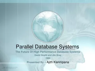
Parallel Database Systems

1. Parallel Database Systems Mike Carey CS 295 Fall 2011 Taken/tweaked from the Wisconsin DB book slides by Joe Hellerstein (UCB) with much of the material borrowed from Jim Gray (Microsoft Research). See also: http://research.microsoft.com/~Gray/talks/McKay1.ppt

2. Why Parallel Access To Data? At 10 MB/s 1.2 days to scan 1,000 x parallel 1.5 minute to scan. 1 Terabyte Bandwidth 1 Terabyte 10 MB/s Parallelism: Divide a big problem into many smaller ones to be solved in parallel.

3. Parallel DBMS: Intro • Parallelism is natural to DBMS processing • Pipelined parallelism: many machines each doing one step in a multi-step process. • Partitioned parallelism: many machines doing the same thing to different pieces of data. • Both are natural in DBMS! Any Any Sequential Sequential Pipeline Program Program Sequential Any Any Sequential Partition Sequential Sequential Sequential Sequential Program Program outputs split N ways, inputs merge M ways

4. DBMS: The || Success Story • For a long time, DBMSs were the most (only?!) successful/commercial application of parallelism. • Teradata, Tandem vs. Thinking Machines, KSR. • Every major DBMS vendor has some || server. • (Of course we also have Web search engines now. ) • Reasons for success: • Set-oriented processing (= partition ||-ism). • Natural pipelining (relational operators/trees). • Inexpensive hardware can do the trick! • Users/app-programmers don’t need to think in ||

5. Some || Terminology Ideal Xact/sec. (throughput) • Speed-Up • Adding more resources results in proportionally less running time for a fixed amount of data. • Scale-Up • If resources are increased in proportion to an increase in data/problem size, the overall time should remain constant. degree of ||-ism Ideal sec./Xact (response time) degree of ||-ism

6. Shared Memory (SMP) Shared Nothing (network) Shared Disk CLIENTS CLIENTS CLIENTS Processors Memory Architecture Issue: Shared What? Hard to program Cheap to build Easy to scale Easy to program Expensive to build Difficult to scale (Use affinity routing to approximate SN- like non-contention) VMScluster, Sysplex Sequent, SGI, Sun Tandem, Teradata, SP2

7. What Systems Work This Way (as of 9/1995) • Shared Nothing • Teradata: 400 nodes • Tandem: 110 nodes • IBM / SP2 / DB2: 128 nodes • Informix/SP2 48 nodes • ATT & Sybase ? nodes • Shared Disk • Oracle 170 nodes • DEC Rdb 24 nodes • Shared Memory • Informix 9 nodes • RedBrick ? nodes

8. Different Types of DBMS ||-ism • Intra-operator parallelism • get all machines working together to compute a given operation (scan, sort, join) • Inter-operator parallelism • each operator may run concurrently on a different site (exploits pipelining) • Inter-query parallelism • different queries run on different sites • We’ll focus mainly on intra-operator ||-ism

9. Automatic Data Partitioning Partitioning a table: RangeHashRound Robin A...E F...J F...J T...Z T...Z K...N K...N O...S T...Z F...J K...N O...S A...E O...S A...E Good for equijoins, exact-match queries, and range queries Good for equijoins, exact match queries Good to spread load Shared disk and memory less sensitive to partitioning. Shared nothing benefits from "good" partitioning.

10. Parallel Scans/Selects • Scan in parallel and merge (a.k.a. union all). • Selection may not require all sites for range or hash partitioning, but always does for RR. • Indexes can be constructed on each partition. • Indexes useful for local accesses, as expected. • However, what about unique indexes...? (May not always want primary key partitioning!)

11. A..C G...M D..F S.. N...R Secondary Indexes • Secondary indexes become a bit troublesome in the face of partitioning... • Can partition them via base table key. • Inserts local (unless unique??). • Lookups go to ALL indexes. • Can partition by secondary key ranges. • Inserts then hit 2 nodes (base, index). • Ditto for index lookups (index, base). • Uniqueness is easy, however. • Teradata’s index partitioning solution: • Partition non-unique by base table key. • Partition unique by secondary key. A..Z A..Z A..Z A..Z A..Z Base Table Base Table

12. Partitions OUTPUT 1 1 INPUT 2 2 hash function h . . . Original Relations (R then S) B-1 B-1 B main memory buffers Disk Disk Grace Hash Join • In Phase 1 in the parallel case, partitions will get distributed to different sites: • A good hash function automatically distributes work evenly! (Diff hash fn for partitioning, BTW.) • Do Phase 2 (the actual joining) at each site. • Almost always the winner for equi-joins. Phase 1

13. Dataflow Network for || Joins • Use of split/merge makes it easier to build parallel versions of sequential join code.

14. Parallel Sorting • Basic idea: • Scan in parallel, range-partition as you go. • As tuples arrive, perform “local” sorting. • Resulting data is sorted and range-partitioned (i.e., spread across system in known way). • Problem:skew! • Solution: “sample” the data at the outset to determine good range partition points.

15. Parallel Aggregation • For each aggregate function, need a decomposition: • count(S) = Scount(s(i)), ditto for sum() • avg(S) = (Ssum(s(i))) /Scount(s(i)) • and so on... • For groups: • Sub-aggregate groups close to the source. • Pass each sub-aggregate to its group’s partition site.

16. A B R S Complex Parallel Query Plans • Complex Queries: Inter-Operator parallelism • Pipelining between operators: • note that sort or phase 1 of hash-join block the pipeline! • Bushy Trees Sites 1-8 Sites 1-4 Sites 5-8

17. Observations • It is relatively easy to build a fast parallel query executor. • S.M.O.P., well understood today. • It is hard to write a robust and world-class parallel query optimizer. • There are many tricks. • One quickly hits the complexity barrier. • Many resources to consider simultaneously (CPU, disk, memory, network).

18. Parallel Query Optimization • Common approach: 2 phases • Pick best sequential plan (System R algorithm) • Pick degree of parallelism based on current system parameters. • “Bind” operators to processors • Take query tree, “decorate” it with site assignments as in previous picture.

19. What’s Wrong With That? • Best serial plan != Best || plan! Why? • Trivial counter-example: • Table partitioned with local secondary index at two nodes • Range query: all of node 1 and 1% of node 2. • Node 1 should do a scan of its partition. • Node 2 should use secondary index. • SELECT * FROM telephone_book WHERE name < “NoGood”; Index Scan Table Scan N..Z A..M

20. Parallel DBMS Summary • ||-ism natural to query processing: • Both pipeline and partition ||-ism! • Shared-Nothing vs. Shared-Memory • Shared-disk too, but less “standard” (~older...) • Shared-memory easy, costly. Doesn’t scaleup. • Shared-nothing cheap, scales well, harder to implement. • Intra-op, Inter-op, & Inter-query ||-ism all possible.

21. || DBMS Summary, cont. • Data layout choices important! • In practice, will not N-way partition every table. • Most DB operations can be done partition-|| • Select, sort-merge join, hash-join. • Sorting, aggregation, ... • Complex plans. • Allow for pipeline-||ism, but sorts and hashes block the pipeline. • Partition ||-ism achieved via bushy trees.

22. || DBMS Summary, cont. • Hardest part of the equation: optimization. • 2-phase optimization simplest, but can be ineffective. • More complex schemes still at the research stage. • We haven’t said anything about xacts, logging, etc. • Easy in shared-memory architecture. • Takes a bit more care in shared-nothing architecture

23. || DBMS Challenges (mid-1990’s) • Parallel query optimization. • Physical database design. • Mixing batch & OLTP activities. • Resource management and concurrency challenges for DSS queries versus OLTP queries/updates. • Also online, incremental, parallel, and recoverable utilities for load, dump, and various DB reorg ops. • Application program parallelism. • MapReduce, anyone...? • (Some new-ish companies looking at this, e.g., GreenPlum, AsterData, …)