Optimized Algorithms for Data Analysis in Parallel Database Systems
This research outlines advanced algorithms for analyzing data in parallel database systems, addressing challenges in model computation and graph analytics integration. The study explores Linear Models with Parallel Matrix Multiplication and Graph Analytics with Parallel Matrix-Matrix and Matrix-Vector Multiplication for efficient data processing. The motivation stems from handling large and continuously growing datasets with enhanced security measures. The contributions include advanced modeling techniques and graph analysis methods integrated into parallel database systems, enhancing efficiency and performance. The research timeline showcases key works in Linear Models and Graph Analytics, providing insights into improving data analysis in parallel databases.

Optimized Algorithms for Data Analysis in Parallel Database Systems
E N D
Presentation Transcript
Optimized Algorithms for Data Analysis in Parallel Database Systems Wellington M. Cabrera Advisor: Dr. Carlos Ordonez
Outline • Motivation • Background • Parallel DBMSs under shared-nothing architecture • Data sets • Review of work pre proposal • Linear Models with Parallel Matrix Multiplication • Variable Selection, Linear Regression, PCA • Presentation of recent work • Graph Analytics with Parallel Matrix-Matrix Multiplication • Transitive closure, All Pairs Shortest Path, Triangle Counting • Graph Analytics with Parallel Matrix-Vector Multiplication • PageRank, Connected Components • Reachability, SSSP • Conclusions
Motivation • Large datasets found in any domain. • Continuous growing of data. • Number of records • Number of attributes/features • DBMS are systems with a lot of research behind. • Query optimizer • Optimized I/O • Parallelism • DBMS offer increased security, compared with ad-hoc file management.
Issues • Most of the data analysis, model computation and graph analytics is done outside of the database, exporting CSV files. • It is difficult to express complex models and graph algorithms in a DBMS. • No matrix operations support • Queries may become hard to program • Algorithms programmed without a deep understanding of DBMS technology may run with a poor performance. • What’s wrong with exporting the data set to external systems? • Data Privacy threat • Waste of time • Analysis is delayed
Contributions History/Timeline • First part of PhD • Linear Models with Parallel Matrix Multiplication 1, 2 • Variable Selection, Linear Regression, PCA • Second part of PhD • Graph Analytics with Parallel Matrix-Matrix Multiplication3 • Transitive closure, All Pairs Shortest Path, Triangle Counting • Graph Analytics with Parallel Matrix-Vector Multiplication4 • PageRank, Connected Components • Reachability, SSSP 1. The Gamma Matrix to Summarize Dense and Sparse Data Sets for Big Data Analytics. IEEE TKDE 28(7): 1905-1918 (2016) 2. Accelerating a Gibbs sampler for variable selection on genomics data with summarization and variable pre-selection combining an array DBMS and R. Machine Learning 102(3): 483-504 (2016) 3. Comparing columnar, row and array DBMSs to process recursive queries on graphs. Inf. Syst. 63: 66-79 (2017) 4. Unified Algorithm to Solve Several Graph Problems with Relational Queries. Alberto Mendelzon International Workshop on Foundations of Data Management (2016)
Definitions • Data set for Linear Models • Let X = {x1, ..., xn}be the input data set with n data points, where each point has d dimensions. • X is a d × n matrix, where the data point xi is represented by a column vector (thus, equivalent to a d× 1 matrix). • Y is a 1 x n vector , representing the dependent variable . • Generally n>d; therefor X is a rectangular matrix • Big data: n>>d
Definition: Graph data set • LetG=(V,E) m=|E| ; n =|V| We denominate the adjacency matrix of G as E . E is a n x n matrix, generally sparse • S: a vector of vertices used in graph computations |S|=|V|=n • Each entry Si represents a vertex attribute. • distance from an specific source, membership, probability • We omit values in S with no information (like ∞ for distances, 0 for probabilities) • Notice Eisn x n , but Xisd x n
DBMS Storage classes • Row Store: Legacy, transactions • Column Store: Modern, analytics • Array Store: Emerging, Scientific
Linear Models: data set storage in columnar/row DBMS • Case n>>d • Low and high dimensional datasets • n in millions/billions; d up to few hundreds • Most data sets: marketing, public health, sensor networks. • data point xi stored as a row, with d columns • extra column to store outcome Y • Thus, data set is stored as a table T, where T has n rows and d+1 columns. • Parallel databases may partition T either by hash function or mod function.
Linear Models: data set storage in columnar/row DBMS • Case d>n • Very High d, low n. • d in thousands. Examples: • Gene expression (microarray) data. • Word frequency in documents • Cannot keep n>d layout. Number of columns beyond most Row DBMS limits. • Data point xi stored as a column • Extra row to store the outcome Y • Thus, data set is stored in a table T, which has n columns and d+1 rows
Linear Models: data set representation in an array DBMS • Array databases store data as multidimensional arrays, instead of relational tables. • Arrays are partitioned by chunks (bi-dimensional data blocks) • All chunks in a specific array have the same shape and size. • Data points xi stored as rows, with an extra column for the outcome yi • Thus, the dataset is represented as a bi-dimensional array, with n rows and d+1 columns.
Graph data set • Row and columnar DBMS: E(i,j,v) • Array DBMS: E as a n x n sparse array
Gamma Matrix Γ= Z ZT
Models Computation • 2-Step algorithm for PCA, LR, VS…. One pass to the dataset. • Compute summarization matrix (Gamma) in one pass. • Compute models (PCA, LR, VS) using Gamma. • Preselection & 2-Step algorithm for very high-dimensional VS ( Two passes). A preprocess step is incorporated • Compute partial Gamma and perform preselection. • Compute summarization matrix (Gamma) in one pass. • Compute VS using Gamma.
Models Computation • 2-step algorithm • Compute the summarization matrix Gamma in the DBMS ( cluster, multiple nodes/cores) • Compute the model locally exploiting Gamma and parallel matrix operations (LAPACK) , using any programming language (i.e. R, C++, C#). • This approach was published in our work [1]
First step: One pass data set summarization • We introduced the Gamma Matrix in [1]. • The Gamma Matrix ( or Г) is a square matrix with d+2 rows and columns that contains a set of sufficient statistics, useful to compute several statistical indicators and models. • PCA, VS, LR, covariance/correlation matrices. • Computed in parallel with multiple cores or multiple nodes.
Matrix Multiplication Z∙ZT • Parallel Computation with Multicore CPU (single node) in one pass. • AGGUDF are processed in parallel, in four phases (initialize, accumulate, merge, terminate) and enable multicore processing. • Initialize: Variables set up • Accumulate: partial Gammas are calculated via vector products. • Merge: Final Gamma is computed by adding partial Gammas. • Terminate: Control returns to main processing • Computation with LAPACK ( main memory) • Computation with OpenMPI
Matrix Multiplication Z∙ZT • Parallel Computation with multiple nodes • Computation in Parallel Array Database. • Each worker can process with one or multiple cores. • Each core computes its own partial Gamma, using its own local data. • Master node receives partial Gammas from workers • Master node computes final Gamma with matrix addition.
Models Computation • Contribution summary; • Enables the analysis of very high dimensional data sets in the DBMS. • Overcomes the problem of data sets larger than RAM (d< n) • 10s to 100s times faster than standard approach
PCA • Compute Г, which contains n, L and Q • Compute ρ, solve SVD of ρ, and select the k principal components
Variable Selection1 + 2 Step Algorithm • Pre-selection • Based on marginal correlation ranking • Calculate correlation between each variable and the outcome • Sort in descending order • Take the best d variables • Top d variables are considered for further analysis • Compute Г, which contains Qγ and XγYT • Iterate the Gibbs sampler a sufficiently large number of iterations to explore
Optimizing Gibbs Sampler • Non-conjugate Gaussian priors require the full Markov Chain. • Conjugate priors simplify the computation. • β,σintegrated out. • Marin-Roberts formulation • Zellner-g prior for βand Jeffrey’s prior for σ
PCA DBMS : SciDB System : Local 1 node, 2 instances Dataset: KDDnet
LR DBMS : SciDB System : Local 1 node, 2 instances Dataset: KDDnet
VS DBMS : SciDB System : Local 1 node, 2 instances Dataset: Brain Cancer - miRNA DBMS : SciDB System : Local 1 node, 2 instances Dataset: Brain Cancer - miRNA
Optimizing Parallel JoinData Partitioning • Join locality: E, S partitioned by hashing in the joining columns. • Sorted tables: a merge join is possible, complexity O(n)
Optimizing Parallel JoinData Partitioning • S split in N chunks • E split in N x N squared chunks
Handling Skewed data • Chunk density for a social network data set in a 8 instances cluster. • Skewness results on uneven data distribution (right) • Chunk density after repartition (left) • Edges per worker, before (right) and after (left) repartitioning
Unified Algorithm • Unified Algorithm solves: • Reachability from a source vertex, SSSP • WCC, Page Rank
Data Partitioning in Array DBMS • Data is partitioned by chunks: ranges • Vector S is evenly partitioned through the cluster. • Sensible to skewness • Redistribution using mod function
Experimental Validation • Time complexity close to linear • Comparing with a classical optimization: • Replication of the smallest table
Experimental Validation • Optimized Queries in array DBMS vs ScaLAPACK
Experimental Validation • Speed up with real data sets
Matrix Multiplication with SQL Queries • Matrix-Matrix Multiplication (+ , x ) semiring SELECT R.i, E.j, sum(R.v * E.v) FROM R join E on R.j=E.i GROUP BY i, j • Matrix-Matrix Multiplication (min , - ) semiring SELECT R.i, E.j, min(R.v + E.v) FROM R join E on R.j=E.i GROUP BY i, j
Data partitioning for parallel computation in Array DBMS • Distributed storage of R, E in array DBMS