The Arbitrage Pricing Theory and Multifactor Models of Risk and Return

1. The Arbitrage Pricing Theory and Multifactor Models of Risk and Return P.V. Viswanath For a First Course in INvestments

2. Learning Goals • Why do we need multi-factor models? • How are the multi-factor models grounded in the CAPM/APT? • What is the APT? • How does the APT differ from the CAPM? • How can we understand the Fama-French factor models?

3. Why multi-factor models? • As a conceptual model, the CAPM is very useful. However, in practice, with the data and methods that are available to us to measure market beta, it is not sufficiently useful to compute required rates of return and expected returnsor to discover mispriced securities. • Multifactor models are useful in this context. • These models introduce uncertainty stemming from multiple sources, whereas the CAPM, in principle, limits risk to one source – covariance with the market portfolio.

4. Using the CAPM as a basis for factor models • In the CAPM, the only relevant factor is the market model. However, the market factor itself could be composed of different macroeconomic factors, e.g. business cycle uncertainty , interest rates, inflation etc. • Suppose the market is composed of two factors F1 and F2, i.e. Rm= sF1 + (1-s)F2, where even though we can’t observe Rm, we can observe F1 and F2. • Then we can rewrite the CAPM as:E(Ri) = Rf + b[Rm-Rf] = (1-b)Rf+ bE(Rm) = (1-b)Rf + b[sE(F1) + (1-s)E(F2)]; rewriting, E(Ri) = Rf + bs [E(F1) - Rf ]+ b(1-s)[E(F2) - Rf]. • This suggests a regression of Rion (F1 - Rf)and (F2 - Rf):E(Ri) = Rf + gi1[E(F1)-Rf] + gi2[E(F2)-Rf]. • The two sources of risk here are exposure to the two factors; comparing the two equations, we also see the implication that gi1 + gi2 = b. • In this formulation, we don’t need to observe the market portfolio any more. • However the factors must be observable, and our market portfolio decomposition is assumed to be correct.

5. The APT approach • The following description assumes two factors, but there could be many factors in principle. • Assume that returns can be generated as in a quasi-market model: Ri= ai + bi1F1 + bi2F2 + error. • If there are enough assets that are sufficiently different from each other, it should be possible to create three well-diversified portfolios that had no uncertainty other than their exposure to F1 and F2 (i.e. the error term would be zero). • Then, the expected return on these three portfolios can be described by a linear combination of their b’s:E(R) = c0 + c1 bi1 + c2 bi2. • We can see this by means of an example.

6. The APT approach • Suppose these three portfolios – let’s call them A, B and C – were described by the following parameters: • As we concluded above, E(R) = c0 + c1 bi1 + c2 bi2. • That is, 15 = c0 + 1c1 + 0.6c214 = c0 + 0.5c1 + 1.0c2 and 10 = c0 + 0.3c1 + 0.2c2. • Solving this system of three equations for c0, c1 and c2, we find c0 = 7.75, c1 = 5 and c2 = 3.75. • The claim is that this pricing equation (E(R) = 7.75 + 5 bi1 + 3.75 bi2) can be used to price any security in the economy.

7. The APT approach • Suppose a security, D, exists with bi1 = 0.6 and bi2 = 0.6. Since we have enough securities, we can create a diversified portfolio with almost no idiosyncratic error that would also have the same values for bi1 and bi2. So let’s assume that our security has no idiosyncratic error. • Then, according to our equation, its expected return should be 7.75 + 5 (0.6) + 3.75 (0.6) = 13%. Suppose, however, that the expected return for D is 15%. • Then we can create a combination of securities A, B and C such that this new portfolio, E, has the same b-values as D. • This can be done by solving the system of equations: x1(1.0) + x2(0.5) + x3(0.3) = 0.6; x1(0.6) + x2(1.0) + x3(0.2) = 0.6; x1+x2+x3=1, where the xis are the portfolio weights for portfolio E. In this case, the solution is x1=x2=x3=1/3. This portfolio would have the same b-values as D, but would have an expected return of (15+14+10)/3 = 13%. • Hence an arbitrage opportunity exists. • In general, the exercise of such arbitrage opportunities will force all security prices to be such that expected returns are described by our single pricing equation, E(R) = c0 + c1 bi1 + c2 bi2.

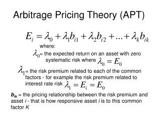
8. The APT approach • We now simplify this pricing equation by identifying c0, c1and c2. • Note that a portfolio with no b-risk will have to earn c0; hence c0 = the risk-free rate. • A portfolio with b1 risk equal to 1 and no b2 risk will earn c0 + c1. Similarly, a portfolio with b2=1 and b1=0 will earn c0+c2. • Hence our pricing equation becomes: E(R) = Rf + [E(RF1)-Rf]bi1 + [E(RF2)-Rf]bi2, where E(RF1) is the expected return on a security or portfolio that has b1=1, b2=0, and E(RF2) is the expected return on a security/portfolio that has b1=0, b2=1.

9. The APT • We can’t guarantee that at all times, all assets will satisfy this equation, since it’s not an equilibrium condition anymore, but rather a no-arbitrage condition. • On the other hand, the advantage of the APT is that we don’t need to worry about the market portfolio anymore. We don’t have the problem of Roll’s critique. • The APT is a purely empirical model – as such, it can be used for a subset of assets in the economy. • So, if we can assert that returns on our subset of assets can be described as Ri= ai + gi1F1 + gi2F2 + error for some F1 and F2, then the APT holds, as long as there are sufficiently many assets in this microcosm. • The problem is that the underlying model could change at any time; we have no guidance as to what generates the underlying model!

10. CAPM versus APT APT CAPM • Model is based on an inherently unobservable “market” portfolio. • Rests on mean-variance efficiency. The actions of many small investors restore CAPM equilibrium. • CAPM describes equilibrium for all assets. • Equilibrium means no arbitrage opportunities. • APT equilibrium is quickly restored even if only a few investors recognize an arbitrage opportunity. • The expected return–beta relationship can be derived without using the true market portfolio.

11. Factor Models • Chen, Roll, and Ross used industrial production, expected inflation, unanticipated inflation, excess return on corporate bonds, and excess return on government bonds. • The Fama-French-Carhart (FFC) model uses firm characteristics – it specifies four different factor portfolios. • The market portfolio • A self-financing portfolio consisting of long positions in small stocks financed by short positions in large stocks – the SMB (small-minus-big) portfolio. • A self-financing portfolio consisting of long positions in stocks with high book-to-market ratios financed by short positions in stocks with low book-to-market ratios – the HML (high-minus-low) portfolio. • A self-financing portfolio consisting of long positions in the top 30% of stocks that did well the previous year financed by short positions the bottom 30% stocks – the PR1YR (prior 1-yr momentum) portfolio. • The resulting factor-pricing equation is: • Since the last three portfolios are self-financing, there is no investment and the risk-free return does not figure in the formula.

12. Using the FFC Model • We see above estimates of expected risk premiums for the four FFC factors. • Let us now consider how to use the FFC model in practice. Suppose you find yourself in the situation described below:

13. Using the FFC Model

14. The Fama-French model • The three factor Fama-French model includes only the market, the SMB and the HML factors. • As points of reference, the historical average from July 1926 to July 2002 of the annual SMB factor has been approximately 3.3%1; and in a recent lecture, in 2003, Ken French stated that he believes the annual SMB premium to be in the range of 1.5-2.0% today. • Over the time period from 1926 to 2002, the premium for value stocks (HML factor) has averaged approximately 5.1% annually, and was cited by Ken French in 2003 as having a current value of approximately 3.5-4.0%.