Download

1 / 45
470 likes | 558 Vues
Learn how Index Models and the Arbitrage Pricing Theory offer solutions in finance, addressing estimation problems, CAPM shortcomings, stock returns, and more. Explore the benefits, costs, and risks associated with these models.

E N D
Index Models and APT Provide Potential Solutions To: • Estimation problems in implementing MPT • Shortcomings of CAPM
Single Index Model (SIM) • Stock’s Rate of Return • Percentage change in the index (I) • Common factor • Changes related to firm-specific events (ei) • On average = 0 • Any given period, it can be + or -
SIM Calculations • Ri = Constant + Common-Factor + Firm-Specific News News • Ri = i + iI + ei • I = Ri - iI • Note: CAPM is a specific form of SIM
The Return Components Ri Realized Return Firm-Specific News Average Return With Common-Factor News i i I
Why Does SIM Reduce Computations? • It Decreases the Number of Calculations of Covariances • From Cov(Ri, Rj) = Cov(i+ iI + ei,j +jI + ej) • To Cov (Ri, Rj) = i j2I • Because (by assumption) Cov(ei, ej) = 0 and Cov(I, ei) = 0
Estimation Issues • Results of portfolio allocation depend on accurate statistical inputs • Estimates of • Expected returns • Standard deviation • Correlation coefficient • Among entire set of assets • With 100 assets, 4,950 correlation estimates • Estimation risk refers to potential errors
Estimation Issues • With the assumption that stock returns can be described by a single market model, the number of estimated inputs required for the covariances reduces to the number of assets (one beta for each) plus one (the variance of the Index’s return) • No. of estimated inputs required for covariances:
Estimation Issues • Benefits of using SIM for estimating Eff. Frontier • Fewer estimated inputs implies less chance for estimation error (true Eff. Frontier is more likely to be near where it is estimated to be) • Costs of using SIM • Potentially unrealistic, oversimplified assumptions • Ignores the potential for “industry effects” • different stocks in the same industry will tend to move together in ways that are separate from what the market as a whole is doing • But, market effects are still the strongest
Systematic Risk Common-Factor Risk Undiversifiable Portfolio Risk Unsystematic Risk Firm-Specific Risk Diversifiable Investors are not rewarded for unsystematic risk
Systematic Risk • Inflation rate • Unemployment rate • Interest rate • Unsystematic Risk • Resignation of the president • Change in dividends • New discovery
Return On A Portfolio Portfolio + Portfolio Return + Portfolio Return Intercept Due to Due to Market Factor Firm-Specific Factors
Risk And E(R) With SIM Start With E(Ri) = I + i E(I) + E(ei)
With Diversification 2 Unsystematic Risk Systematic Risk n 30
Risk And E(R) With SIM E(ei) = 0 Ri = E(Ri) + I[I - E(I)] + ei Just Like APT
APT • Linear Risk-Return Relationship • No Arbitrage Opportunities • Equilibrium Model
What Is Arbitrage? • Borrow at 5% and Save at 6% • Simultaneously buying stock cheaply on one market and selling it short on another higher-quoted market • What Causes the Arbitrage? • Zero out-of-pocket investment • Return is always nonnegative
Arbitrage Pricing Theory (APT) • Arbitrage is a process of buying a lower priced asset and selling a higher priced asset, both of similar risk, and capturing the difference in arbitrage profits • The general arbitrage principle states that two identical securities will sell at identical prices • Price differences will immediately disappear as arbitrage takes place
Arbitrage Pricing Theory (APT) • CAPM is criticized because of the difficulties in selecting a proxy for the market portfolio as a benchmark • An alternative pricing theory with fewer assumptions was developed: • Arbitrage Pricing Theory
Assumptions of Arbitrage Pricing Theory (APT) 1. Capital markets are perfectly competitive 2. Investors always prefer more wealth to less wealth with certainty 3. The stochastic process generating asset returns can be presented as K factor model • Common factors plus some noise • Describes the risk-return relationship • Other Assumptions: • Large number of assets in the economy • Short sales allowed with proceeds
Assumptions of CAPMThat Were Not Required by APT APT does not assume • A market portfolio that contains all risky assets, and is mean-variance efficient • Normally distributed security returns • Quadratic utility function
Arbitrage Pricing Theory (APT) For i = 1 to N where: Ri = return on asset i during a specified time period Ei = expected return for asset i bik = reaction in asset i’s returns to movements in the kth common factor δk = a common factor with a zero mean that influences the returns on all assets εi = a unique effect on asset i’s return that, by assumption, is completely diversifiable in large portfolios and has a mean of zero N = number of assets
Arbitrage Pricing Theory (APT) Multiple factors expected to have an impact on all assets:
Arbitrage Pricing Theory (APT) Multiple factors expected to have an impact on all assets: • Inflation
Arbitrage Pricing Theory (APT) Multiple factors expected to have an impact on all assets: • Inflation • Growth in GNP
Arbitrage Pricing Theory (APT) Multiple factors expected to have an impact on all assets: • Inflation • Growth in GNP • Major political upheavals
Arbitrage Pricing Theory (APT) Multiple factors expected to have an impact on all assets: • Inflation • Growth in GNP • Major political upheavals • Changes in interest rates
Arbitrage Pricing Theory (APT) Multiple factors expected to have an impact on all assets: • Inflation • Growth in GNP • Major political upheavals • Changes in interest rates • And many more….
Arbitrage Pricing Theory (APT) Multiple factors expected to have an impact on all assets: • Inflation • Growth in GNP • Major political upheavals • Changes in interest rates • And many more…. Contrast with CAPM insistence that only beta is relevant
Arbitrage Pricing Theory (APT) bik(beta(i,k)) determines how each asset reacts to this common factor Each asset may be affected by growth in GNP, but the effects will differ In application of the theory, the factors are not identified Similar to the CAPM, the unique effects ( εi ) are independent and will be diversified away in a large portfolio
APT’s Common Factors • Used I - E(I) Instead of Just I • Called the Surprise Factor • Measures the Difference Between • Expectations • Actual outcomes
Firm’s Beta The Larger the Beta The Larger the Effect of the Surprise On the Firm’s Return
Arbitrage Pricing Theory (APT) • APT assumes that, in equilibrium, the return on a zero-investment, zero-systematic-risk portfolio is zero when the unique effects are diversified away • The expected return on any asset i (Ei) can be expressed as:
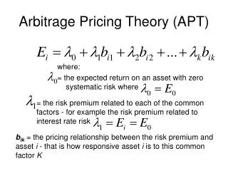
Arbitrage Pricing Theory (APT) where: = the expected return on an asset with zero systematic risk: = the risk premium related to each of the common factors - for example the risk premium related to interest rate risk bik = the pricing relationship between the risk premium and asset i - that is how responsive asset i is to this common factor k
Example of Two Stocks and a Two-Factor Model λ0= the rate of return on a zero-systematic-risk asset (zero beta: bik=0) is 3 percent ( λ0 = 0.03 ) λ1= changes in the rate of inflation. The risk premium related to this factor is 1 percent for every 1 percent change in the rate ( λ1 = 0.01 ) λ2= percent growth in real GNP. The average risk premium related to this factor is 2 percent for every 1 percent change in the rate ( λ2 = 0.02 )
Example of Two Stocks and a Two-Factor Model = the response of asset X to changes in the rate of inflation is 0.50 = the response of asset Y to changes in the rate of inflation is 2.00 = the response of asset X to changes in the growth rate of real GNP is 1.50 = the response of asset Y to changes in the growth rate of real GNP is 1.75
Example of Two Stocks and a Two-Factor Model = .03 + (.01)bi1 + (.02)bi2 Ex = .03 + (.01)(0.50) + (.02)(1.50) = .065 = 6.5% Ey = .03 + (.01)(2.00) + (.02)(1.75) = .085 = 8.5%
APT vs. CAPM • Similar Results • Both yield a linear risk-return relationship • Advantage of APT • More realistic, less restrictive assumptions • Allows for multiple risk factors (e.g., industry effects) • Disadvantage of APT • Fails to identify common factors
Multifactor APT • Suggested Factors • Default premium • Term structure • Inflation • Corporate profits • Market risk • E(Ri) = λ0 + λ1i1 + λ2i2 + … + λkik
Empirical Tests of the APT • Studies by Roll and Ross and by Chen support APT by explaining different rates of return with some better results than CAPM • Reinganum’s study did not explain small-firm results • Dhrymes and Shanken question the usefulness of APT because it was not possible to identify the factors
Roll-Ross Study 1. Estimate the expected returns and the factor coefficients from time-series data on individual asset returns 2. Use these estimates to test the basic cross-sectional pricing conclusion implied by the APT
Extensions of the Roll-Ross Study • Cho, Elton, and Gruber examined the number of factors in the return-generating process that were priced • Dhrymes, Friend, and Gultekin (DFG) reexamined techniques and their limitations and found the number of factors varies with the size of the portfolio
The APT and Anomalies • Small-firm effect Reinganum - results inconsistent with the APT Chen - supported the APT model over CAPM • January anomaly Gultekin - APT not better than CAPM Burmeister and McElroy - effect not captured by model, but still rejected CAPM in favor of APT • APT and inflation Elton, Gruber, and Rentzler - analyzed real returns
The Shanken Challenge to Testability of the APT • If returns are not explained by a model, it is not considered rejection of a model; however if the factors do explain returns, it is considered support • APT has no advantage because the factors need not be observable, so equivalent sets may conform to different factor structures • Empirical formulation of the APT may yield different implications regarding the expected returns for a given set of securities • Thus, the theory cannot explain differential returns between securities because it cannot identify the relevant factor structure that explains the differential returns
Alternative Testing Techniques • Jobson proposes APT testing with a multivariate linear regression model • Brown and Weinstein propose using a bilinear paradigm • Others propose new methodologies