The Arbitrage Pricing Theory (Chapter 10)
450 likes | 2.28k Vues
The Arbitrage Pricing Theory (Chapter 10). Single-Factor APT Model Multi-Factor APT Models Arbitrage Opportunities Disequilibrium in APT Is APT Testable? Consistency of APT and CAPM. Essence of the Arbitrage Pricing Theory.

The Arbitrage Pricing Theory (Chapter 10)
E N D
Presentation Transcript
The Arbitrage Pricing Theory(Chapter 10) • Single-Factor APT Model • Multi-Factor APT Models • Arbitrage Opportunities • Disequilibrium in APT • Is APT Testable? • Consistency of APT and CAPM
Essence of the Arbitrage Pricing Theory • Given the impossibility of empirically verifying the CAPM, an alternative model of asset pricing called the Arbitrage Pricing Theory (APT) has been introduced. • Essence of APT • A security’s expected return and risk are directly related to its sensitivities to changes in one or more factors (e.g., inflation, interest rates, productivity, etc.)
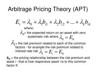
Essence of the Arbitrage Pricing Theory(Continued) • In other words, security returns are generated by a single-index (one factor) model: where: • or, by a multi-index (multi-factor) model:
CAPM (Zero Beta Version) Factor = Market Portfolio Actual Returns: Expected Returns: APT (One Factor Version) Factor = “Your Choice” Actual Returns: Expected Returns: Single-Factor APT Model(A Comparison With the CAPM)
CAPM (Zero Beta Version) Continued Portfolio Variance: APT (One Factor Version) Continued Portfolio Variance: Single-Factor APT Model(A Comparison With the CAPM)Continued
Multi-Factor APT Models • One Factor • Two Factors
Multi-Factor APT Models(Continued) • N Factors
The Ideal APT Model Ideally, you wish to have a model where all of the covariances between the rates of return to the securities are attributable to the effects of the factors. The covariances between the residuals of the individual securities, Cov(j, k), are assumed to be equal to zero.
APT With an Unlimited Number of Securities Given an infinite number of securities, if security returns are generated by a process equivalent to that of a linear single-factor or multi-factor model, it is impossible to construct two different portfolios, both having zero variance (i.e., zero betas and zero residual variance) with two different expected rates of return. In other words, pure riskless arbitrage opportunities are not available.
Pure Riskless Arbitrage Opportunities(An Example) Note: If two zero variance portfolios could be constructed with two different expected rates of return, we could sell short the one with the lower return, and invest the proceeds in the one with the higher return, and make a pure riskless profit with no capital commitment.
Pure Riskless Arbitrage Opportunities(An Example) - Continued Expected Return (%) D C B A E(rZ)1 E(rZ)2 Factor Beta
“Approximately Linear” APT Equations • The APT equations are expressed as being “approximately linear.” That is, the absence of arbitrage opportunities does not ensure exact linear pricing. There may be a few securities with expected returns greater than, or less than, those specified by the APT equation. However, because their number is fewer than that required to drive residual variance of the portfolio to zero, we no longer have a riskless arbitrage opportunity, and no market pressure forcing their expected returns to conform to the APT equation.
Disequilibrium Situation in APT: A One Factor Model Example • Portfolio (P) contains 1/2 of security (B) plus 1/2 of the zero beta portfolio: • Portfolio (P) dominates security (A). (i.e., it has the same beta, but more expected return). Expected Return (%) B P E(rP) E(I1) Equilibrium Line E(rA) A E(rZ) Beta
Disequilibrium Situation in APT: A One Factor Model Example(Continued) • Arbitrage: Investors will sell security (A). Price of security (A) will fall causing E(rA) to rise. Investors will use proceeds of sale of security (A) to purchase security (B). Price of security (B) will rise causing E(rB) to fall. Arbitrage opportunities will no longer exist when all assets lie on the same straight line.
Anticipated Versus Unanticipated Events • Given a Single-Factor Model: • Substituting the right hand side of Equation #2 for Aj in Equation #1:
Anticipated Versus Unanticipated Events(Continued) • Note: If the actual factor value (I1,t) is exactly equal to the expected factor value, E(I1), and the residual (j,t) equals zero as expected, then all return would have been anticipated: rj,t = E(rj) If (I1,t) is not equal to E(I1), or (j,t) is not equal to zero, then some unanticipated return (positive or negative) will be received.
Anticipated Versus Unanticipated Events(A Numerical Example) • Given: • Expected Return: • Anticipated Versus Unanticipated Return:
Anticipated Versus Unanticipated Returns(A Graphical Display) rj,t = .115 .105 E(rj) = .09 E(rZ) = .06 .03 E(rZ) I1,t E(I1)
Consistency of the APT and the CAPM I1,t I2,t M,I1 M,I2 AI1 AI2 rM,t rM,t 0 0 • Consider APT for a Two Factor Model: • In terms of the CAPM, we can treat each of the factors in the same manner that individual securities are treated: (See charts above) • CAPM Equation:
Note that M,I1 and M,I2 are the CAPM (market) betas of factors 1 and 2. Therefore, in terms of the CAPM, the expected values of the factors are: By substituting the right hand sides of Equations 1 and 2 for E(I1) and E(I2) in the APT equation, we get:
There are numerous securities that could have the same CAPM beta (M,j), but have different APT betas relative to the factors (1,j and 2,j). Consistency of the APT and CAPM (an example) Given: Factor 1 (Productivity) M,I1 = .5 Factor 2 (Inflation) M,I2 = 1.5
Assuming the market is efficient, all of the securities (1 through 6) will have equal returns on the average over time since they have a CAPM beta of 1.00. However, some would argue that it is not necessarily true that a particular investor would consider all securities with the same expected return and CAPM beta equally desirable. For example, different investors may have different sensitivities to inflation. Note: It is possible for both the CAPM and the multiple factor APT to be valid theories. The problem is to prove it.
Empirical Tests of the APT • Currently, there is no conclusive evidence either supporting or contradicting APT. Furthermore, the number of factors to be included in APT models has varied considerably among studies. In one example, a study reported that most of the covariances between securities could be explained on the basis of unanticipated changes in four factors: • Difference between the yield on a long-term and a short-term treasury bond. • Rate of inflation • Difference between the yields on BB rated corporate bonds and treasury bonds. • Growth rate in industrial production.
Is APT Testable? • Some question whether APT can ever be tested. The theory does not specify the “relevant” factor structure. If a study shows pricing to be consistent with some set of “N” factors, this does not prove that an “N” factor model would be relevant for other security samples as well. If returns are not explained by some “N” factor model, we cannot reject APT. Perhaps the choice of factors was wrong.
Using APT to Predict Return • Haugen presents a test of the predictive power of APT using the following factors: • Monthly return to U.S. T-Bills • Difference between the monthly returns on long-term and short-term U.S. Treasury bonds. • Difference between the monthly returns on long-term U.S. Treasury bonds and low-grade corporate bonds with the same maturity. • Monthly change in consumer price index. • Monthly change in U.S. industrial production. • Dividend to price ratio of the S&P 500.
Haugen presents continued . . . • Using data for 3000 stocks over the period 1980-1997, he found that the APT did appear to have only limited predictive power regarding returns. • He argues that the “arbitrage” process is extremely difficult in practice. Since covariances (betas) must be estimated, there is uncertainty regarding their values in future periods. Therefore, truly risk-free portfolios cannot be created using risky stocks. As a result, pure riskless arbitrage is not readily available limiting the usefulness of APT models in predicting future stock returns.
