Download

1 / 48
510 likes | 538 Vues
Discover the significance of modes of variability for Subseasonal-to-Seasonal predictions, methods for identification and influence on weather patterns. Learn about atmospheric patterns and their impacts on climate variables.

E N D
Modes of variability and teleconnections: Part I Hai Lin Meteorological Research Division, Environment Canada Advanced School and Workshop on S2S ICTP, 23 Nov- 4 Dec 2015
Outlines • What are modes of variability? • Why are they important to S2S predictions? • Methods for identifying modes of variability e.g., Pacific North American (PNA) pattern, North Atlantic Oscillation (NAO) • Tropical modes of variability: ENSO, IOD, MJO, QBO, etc • Extratropical response to tropical heating • MJO-NAO interactions
Modes of variability • Distinct and organized patterns that are somehow oscillatory in time • Different time scales. Normally low-frequency: from weekly to decadal time scales • Influence on weather and other climate variables • Evolution of the modes with time scales of S2S provides sources of S2S predictability • Normally large-scale multiple centers. Sometimes called teleconnection patterns • They can be generated by atmospheric internal dynamics or variability in other climate component (e.g. SST).
Representation of a mode of variability 1) Spatial pattern 2) Temporal variability: index Why are we interested in the spatial structure of the temporal variability? • Spatial structures are indicative of some organized physical effects that we may be able to understand. • Also, if we can predict the amplitude of a given pattern, we can predict something about the atmosphere (or ocean) over the domain covered by the pattern.
Identification of Atmospheric Patterns Two main methods are used to obtain the main patterns of variability: a) One point correlation b) Empirical Orthogonal Functions (EOF) All methods provide a spatial pattern and an index for the mode of variability
The use of correlation maps to obtain patterns of variability
500 mb geopotential height JJA DJF Map showing regions of th Northern Hemisphere where the DJF-averaged 500 hPa heights flctuate the most from year to year. Note the maxima in the North Pacific and the North Atlantic.
Walalce and Gutzler, MWR, 1981 Correlation maps based on mean-monthly 500 hPa height fields in Dec., Jan, and Feb. The different maps simply use different ‘’reference ponts’’ (identifiable by a correlation of one). The Pacific North American pattern is important because associated with significant variance.
The PNA index IPNA = ¼ [ z*(20ºN, 160ºW) – z*(45ºN, 165ºW) + z*(55ºN, 115ºW) – z*(30ºN,85ºW)] z* is the normalized 500hPa geopotential height anomaly
Comparison of the two methods: • Method (a) simple to use. Does not provide information on the relative importance of different patterns so obtained. • The time series of the strength of the patterns is obtained by forming an “index”, based on the main maxima and minima in the pattern. Examples: the PNA and NAO indices. • EOF analysis requires more calculations. It provides information on the relative importance of the patterns • For the PNA and NAO, method (a) yields spatial structures and time variability very similar to the EOF analysis.
PNA pattern Correlation method research.jisao.washington.edu EOF method www.cpc.noaa.gov
Pacific North American(PNA)Impact on DJF air temperature • Spatial signature of surface air temperature during PNA. Composite anomalies, winter near surface temperature. PNA-, PNA+, Courtesy: M. Markovic
Atmospheric pressure pattern during El Nino winter Source: http://www.ec.gc.ca
Pacific-North American (PNA) pattern • On interannual timescales PNA is the most important mode of variability in the North Pacific sector and second most important (next to NAO) in the Northern Hemisphere. • Natural (internal) model of climate variability associated with strong fluctuation of East Asian jet stream. • Exists in winter half year, strong in DJF • Equivalent-barotropical vertical structure • Influences North American weather • Interannual variability of PNA correlated with ENSO
North Atlantic Oscillation (NAO) The North Atlantic Oscillation is a large-scale seesaw in atmospheric mass between the subtropical high-pressure system over the Azores Islands and the subpolar low-pressure system over Iceland. (From American Museum of Natural History website)
The NAO is a climate fluctuation associated with variations in the pressure difference between the Azores High and the Icelandic Low in the Atlantic sector. The NAO measures the strength of the westerly winds blowing across the North Atlantic Ocean between 40°N and 60°N. First identified in 1920s by Sir Gilbert Walker.
Finding the NAO spatial structure • One-point correlation • EOF analysis
65N, 30W: NAO - NCEP Reanalysis, 500 hPa geopotential DJF over 1958-2001. One point correlation. Hurrel et al., 2003
EOF1 20-90N EOF1 Atlantic Sector Hurrel et al., 2003
The NAO • The NAO is one of the most important modes of atmospheric variability in the northern hemisphere • The NAO has a larger amplitude in winter than in summer • Equivalent barotropic vertical structure
TheNAO index — a measure of phase and amplitude • Station-based index: difference between normalized mean winter SLP anomalies at Lisbon, Portugal and Stykkisholmur, Iceland (e.g., Hurrell, 1996) • Principal component (PC) based
The NAO index INAO = P*(Lisbon, Portugal) – P* (Stykkisholmur, Iceland) P* is the normalized mean-sea-level pressure The index is therefore dimensionless
s = P2* – P1* (Hurrell, 1996)
Impact of an extreme positive NAO • A stronger than normal subtropical high pressure centre and a deeper than usual Icelandic low • Stronger westerly winds and storm activity across the Atlantic Ocean • Wetter winter in north-west Europe, drier conditions in Mediterranean region • Warmer winter condition over most of the NH land
How is the NAO variability generated? The NAO is mainly generated by atmospheric internal dynamics: interactions among different scales and frequencies in the atmosphere This implies lack of forecast skill beyond 2 weeks
One important mechanism Convergence of momentum flux by eddies, e.g., baroclinic Rossby waves High-frequency eddies act as a forcing to zonal mean flow
Mechanisms other than internal variability? Some recent studies revealed causes remote to the NAO or external to the extratropical atmosphere: • MJO • SST anomaly in the tropics • Changes in snow cover • Stratospheric influence This implies possibility of some forecast skill beyond 2 weeks. However, such forced signal is very weak comparing to noise.
Other extratropical modes of variability • East Atlantic (EA), western Atlantic (WA), western Pacific (WP), Eurasian pattern (EU), etc (Wallace and Gutzler 1981) • North Annular Mode (NAM) • Southern Annular Mode (SAM) • Pacific Decadal Oscillaiton (PDO)
Tropical modes of variability • El Nino – Southern Oscillation (ENSO) interannual time scale (2-7 years) • Quasi-Biennial Oscillation (QBO) interannual time scales (~28 months) • Indian Ocean Dipole (IOD) interannual to decadal time scale • Madden-Julian Oscillation (MJO) subseasonal time scale (30-60 days)
The Madden-Julian Oscillation (MJO) • Discovered by Madden and Julian (1971). Spectrum analysis of 10 year record of SLP at Canton, and upper level zonal wind at Singapore. Peak at 40-50 days. • Dominant tropical wave on intraseasonal time scale • 30-60 day period, wavenumber 1~3 • propagates eastward along the equator (~5 m/s in eastern Hemisphere, and ~10 m/s in western Hemisphere) • Organizes convection and precipitation
Wavenumber-frequency spectra Observations wavenumber 50 d 25 d 50 d 25 d 10S-10N average, winter half year
W-F spectrum of OLR Method: Wheeler and Kiladis (1999) MJO
Vertical cross section From CPC
3-D structure of the MJO From CPC
Mechanisms of the MJO • Kelvin wave? Where does the energy come from? Slow phase speed. • Wave-CISK, importance of convection. • Evaporation-wind feedback • Interaction between convection and radiation • Most GCMs behave poorly in simulating the MJO Mechanisms not fully understood
MJO index • Different definitions • EOF analysis of tropical variables • OLR, 200-hPa velocity potential, U200, etc • Filtering (30-60 days)
Realtime Multivariate MJO index • Wheeler and Hendon (2004) • 3-D structure: OLR, u850, u200 • 1979-2001, daily, 2.5°x2.5° • Remove seasonal cycle, and interannal variability • Band average between 15°S and 15°N • Normalized by its own zonal averaged standard deviation • Combine the 1-D OLR, u850 and u200 anomalies • EOF analysis
Longitudinal distribution of the leading two EOFs • Wavenumber 1 • Baroclinic vertical structure • EOF1 and EOF2 in quadrature Wheeler and Hendon (2004)
Power spectrum of PC1, PC2, PC3 • PC1 and PC2 have a power spectrum peak 30-80 days, with 65% of total variance in this band Wheeler and Hendon (2004)
RMM1 and RMM2 of 2001 and 2002 • PC1 leads PC2 by 10 days Wheeler and Hendon (2004)
Lag correlation btw RMM1 and itself, and with RMM2 • PC1 leads PC2 by 10 days Wheeler and Hendon (2004)
Realtime Multivariate MJO index data http://www.bom.gov.au/climate/mjo/graphics/rmm.74toRealtime.txt Daily values of RMM1, RMM2, phase, amplitude from 1974.6.1 to present
MJO impact: composite analysis Plot anomalies for different phases of the MJO
Composites of tropical Precipitation rate for 8 MJO phases, according to Wheeler and Hendon index. Xie and Arkin pentad data, 1979-2003
NDJ rainfall anomaly in Australia From: http://www.bom.gov.au/climate/mjo
MJO impact: composite analysis Plot anomalies for different phases of the MJO Local or remote impact Simultaneous or lagged composites