Placement 1
Outline What is Placement? Why Placement? Placement Algorithms Goal Understand placement problem Understand placement algorithms. Placement 1. Determination of component locations cells in standard cells ICs on PC board pins on ICs gates in gate array modules in chip floorplan Goal

Placement 1
E N D
Presentation Transcript
Outline What is Placement? Why Placement? Placement Algorithms Goal Understand placement problem Understand placement algorithms Placement 1
Determination of component locations cells in standard cells ICs on PC board pins on ICs gates in gate array modules in chip floorplan Goal minimize chip/board area minimize routing area minimize unused area minimize wiring length minimize length of critical paths evenly distribute power dissipation minimize crosstalk A C B D E D B C E A What is Placement?
Hand placement impractical 1k-1000k cells in standard cell array Multi-goal optimization placement area routing area delay power symmetry - analog circuits Generation of routing specification placement algorithms generate information for router routing channels in slicing structure Why Placement?
Minimize placement cost according to function want fast but reasonably accurate metrics area total area taken by components and estimated wiring wire length (!= delay) minimum spanning tree Steiner tree half-perimeter of bounding box wiring congestion track density along channels cutset size Objective Functions density: avg. 2.2 peak/avg 1.82 1 2 4 3 1
Add components to initial placement select components strongly connected to placed ones place near strongly connected components Algorithm seedComponents = select components for seed currentPlacement = PLACE(seedComponents, currentPlacement) while all components not placed do selectedComponent = SELECT(currentPlacement) currentPlacement = PLACE(selectedComponent, currentPlacement) endloop results not that good often used for initial starting position for other algorithms O(n2) complexity for n components Cluster Growth Placement Unplaced Components Placed Components
Problem “greedy” approaches only accept “downhill” moves that improve cost function can get stuck in local minima far from global minimum Solution: Simulated Annealing jump out of local minima analogy to real annealing heat allows atoms to jump out of local minima cool slowly so atoms jump enough to get close to global minimum Simulated Annealing
Randomly move components score decreases => accept move score increases => accept move with some probability common function: e-deltaS/t probability decreases over time “Cool” system initial “temperature” t high enough to randomize system decrease temperature - the “annealing schedule” do a bunch of moves between temperature changes Simulated Annealing
t = t0 currentPlacement = randomInitialPlacement currentScore = SCORE(currentPlacement) until freezing point is reached do until equilibrium at current t is reached do selectedComponents = SELECT(atRandom) trialPlacement = MOVE(selectedComponents, atRandom) trialScore = SCORE(trialPlacement) deltaS = trialScore - currentScore if deltaS < 0 then currentScore = trialScore else r = uniformrandom(0,1) if r < e-deltaS/t then currentScore = trialScore currentPlacement = trialPlacement endif endif endloop t = a*t endloop Simulated Annealing Algorithm
Pair Swap cells may be of different size results in cell overlap penalize in cost function final postprocess to remove overlaps Single Cell often causes cell overlap more general Cluster move connected components avoids a lot of unnecessary moves Move Functions for Placement
Annealing Schedule cool fast to minimize CPU time cool slowly to get close to global optimum maintain equilibrium at each temperature exponentially slowly to get global optimum usually a = 0.95 a = e-0.7t is closer to optimal at each temperature do “enough” moves to reach equilibrium stop when nothing moves Cost Function weighted sum of objectives score = w1*WireLength + w2*ChipArea + w3*CellOverlapArea + w4*ChipAspectRatio change weights to emphasize different goals “good” weights found by trial-and-error can also change weights as annealing runs Simulated Annealing Control
Minimizing Move Rejection at high temperature nearly all moves are accepted system is randomized at low temperature nearly all moves are rejected most CPU time is wasted Approaches for Placement range limiters - limit distance of moves far away moves unlikely at lower temperatures only generate acceptable moves moves that improve cost function partitioning example: move cells with positive gain must keep around lots of information cost per move is higher, but less wasted effort Simulated Annealing Improvements
Advantages general-purpose optimization approach finds global optimum easily trade speed for quality can incorporate many cost functions can incorporate complex move functions take advantage of problem structure Disadvantages constraints complicate move and cost functions e.g. preplaced blocks, fixed wire lengths CPU hog Implementations Timberwolf, Cadence, Avant! - standard cell placement ACACIA - analog circuit transistor placement Simulated Annealing Issues