Download

1 / 46
470 likes | 677 Vues
Self-calibration Class 13. Read Chapter 6. Assignment 3. Collect potential matches from all algorithms for all pairs Matlab ASCII format, exchange data Implement RANSAC that uses combined match dataset Compute consistent set of matches and epipolar geometry

E N D
Self-calibrationClass 13 Read Chapter 6
Assignment 3 • Collect potential matches from all algorithms for all pairs • Matlab ASCII format, exchange data • Implement RANSAC that uses combined match dataset • Compute consistent set of matches and epipolar geometry • Report thresholds used, match sets used, number of consistent matches obtained, epipolar geometry, show matches and epipolar geometry (plot some epipolar lines). Due next Tuesday, Nov. 2 naming convention: firstname_ij.dat chris_56.dat http://www.unc.edu/courses/2004fall/comp/290/089/assignment3/ [F,inliers]=FRANSAC([chris_56; brian_56; …])
Papers • Each should present a paper during 20-25 minutes followed by discussion. Partially outside of class schedule to make up for missed classes. (When?) • List of proposed papers will come on-line by Thursday, feel free to propose your own (suggestion: something related to your project). • Make choice by Thursday, assignments will be made in class. • Everybody should have read papers that are being discussed.
Papers http://www.unc.edu/courses/2004fall/comp/290b/089/papers/
Dealing with dominant planar scenes (Pollefeys et al., ECCV‘02) • USaM fails when common features are all in a plane • Solution: part 1 Model selection to detect problem
Dealing with dominant planar scenes (Pollefeys et al., ECCV‘02) • USaM fails when common features are all in a plane • Solution: part 2 Delay ambiguous computations until after self-calibration (couple self-calibration over all 3D parts)
Non-sequential image collections Problem: Features are lost and reinitialized as new features 3792 points Solution: Match with other close views 4.8im/pt 64 images
Relating to more views • For every view i • Extract features • Compute two view geometry i-1/i and matches • Compute pose using robust algorithm • Refine existing structure • Initialize new structure For every view i Extract features Compute two view geometry i-1/i and matches Compute pose using robust algorithm For all close views k Compute two view geometry k/i and matches Infer new 2D-3D matches and add to list Refine pose using all 2D-3D matches Refine existing structure Initialize new structure Problem: find close views in projective frame
Determining close views • If viewpoints are close then most image changes can be modelled through a planar homography • Qualitative distance measure is obtained by looking at the residual error on the best possible planar homography Distance =
Non-sequential image collections (2) 2170 points 3792 points 9.8im/pt 64 images 4.8im/pt 64 images
Hierarchical structure and motion recovery • Compute 2-view • Compute 3-view • Stitch 3-view reconstructions • Merge and refine reconstruction F T H PM
Stitching 3-view reconstructions Different possibilities 1. Align (P2,P3) with (P’1,P’2) 2. Align X,X’ (and C,C’) 3. Minimize reproj. error 4. MLE (merge)
Refining structure and motion • Minimize reprojection error • Maximum Likelyhood Estimation (if error zero-mean Gaussian noise) • Huge problem but can be solved efficiently (Bundle adjustment)
P1 P2 P3 M U1 U2 W U3 WT V 3xn (in general much larger) 12xm Sparse bundle adjustment Non-linear min. requires to solve Jacobian of has sparse block structure im.pts. view 1 Needed for non-linear minimization
U-WV-1WT WT V 3xn 11xm Sparse bundle adjustment • Eliminate dependence of camera/motion parameters on structure parameters Note in general 3n >> 11m Allows much more efficient computations e.g. 100 views,10000 points, solve 1000x1000, not 30000x30000 Often still band diagonal use sparse linear algebra algorithms
Self-calibration • Introduction • Self-calibration • Dual Absolute Quadric • Critical Motion Sequences
Motivation • Avoid explicit calibration procedure • Complex procedure • Need for calibration object • Need to maintain calibration
Motivation • Allow flexible acquisition • No prior calibration necessary • Possibility to vary intrinsics • Use archive footage
Projective ambiguity Reconstruction from uncalibrated images projective ambiguity on reconstruction
Stratification of geometry Projective Affine Metric 15 DOF 7 DOF absolute conic angles, rel.dist. 12 DOF plane at infinity parallelism More general More structure
Constraints ? Scene constraints • Parallellism, vanishing points, horizon, ... • Distances, positions, angles, ... Unknown scene no constraints • Camera extrinsics constraints • Pose, orientation, ... Unknown camera motion no constraints • Camera intrinsics constraints • Focal length, principal point, aspect ratio & skew Perspective camera model too general some constraints
Euclidean projection matrix Factorization of Euclidean projection matrix Intrinsics: (camera geometry) (camera motion) Extrinsics: Note: every projection matrix can be factorized, but only meaningful for euclidean projection matrices
Constraints on intrinsic parameters Constant e.g. fixed camera: Known e.g. rectangular pixels: square pixels: principal point known:
Self-calibration Upgrade from projective structure to metric structure using constraintsonintrinsic camera parameters • Constant intrinsics • Some known intrinsics, others varying • Constraints on intrincs and restricted motion (e.g. pure translation, pure rotation, planar motion) (Faugeras et al. ECCV´92, Hartley´93, Triggs´97, Pollefeys et al. PAMI´99, ...) (Heyden&Astrom CVPR´97, Pollefeys et al. ICCV´98,...) (Moons et al.´94, Hartley ´94, Armstrong ECCV´96, ...)
A counting argument • To go from projective (15DOF) to metric (7DOF) at least 8 constraints are needed • Minimal sequence length should satisfy • Independent of algorithm • Assumes general motion (i.e. not critical)
Outline • Introduction • Self-calibration • Dual Absolute Quadric • Critical Motion Sequences
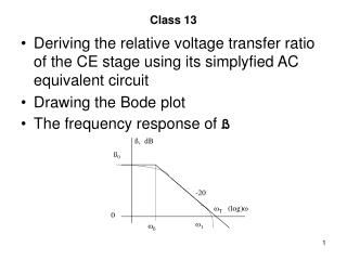
The Dual Absolute Quadric The absolute dual quadric Ω*∞ is a fixed conic under the projective transformation H iff H is a similarity • 8 dof • plane at infinity π∞ is the nullvector of Ω∞ • Angles:
Absolute Dual Quadric and Self-calibration Eliminate extrinsics from equation Equivalent to projection of Dual Abs.Quadric Dual Abs.Quadric also exists in projective world Transforming world so that reduces ambiguity to similarity
* * projection constraints Absolute Dual Quadric and Self-calibration Projection equation: Translate constraints on K through projection equationto constraints on * Absolute conic = calibration object which is always present but can only be observed through constraints on the intrinsics
Constraints on * #constraints condition constraint type
Linear algorithm (Pollefeys et al.,ICCV´98/IJCV´99) Assume everything known, except focal length Yields 4 constraint per image Note that rank-3 constraint is not enforced
Linear algorithm revisited (Pollefeys et al., ECCV‘02) Weighted linear equations assumptions
Projective to metric Compute T from using eigenvalue decomposition of and then obtain metric reconstruction as
Alternatives: (Dual) image of absolute conic • Equivalent to Absolute Dual Quadric • Practical when H can be computed first • Pure rotation(Hartley’94, Agapito et al.’98,’99) • Vanishing points, pure translations, modulus constraint, …
Note that in the absence of skew the IAC can be more practical than the DIAC!
Kruppa equations Limit equations to epipolar geometry Only 2 independent equations per pair But independent of plane at infinity
Refinement • Metric bundle adjustment Enforce constraints or priors on intrinsics during minimization (this is „self-calibration“ for photogrammetrist)
Outline • Introduction • Self-calibration • Dual Absolute Quadric • Critical Motion Sequences
Critical motion sequences (Sturm, CVPR´97, Kahl, ICCV´99, Pollefeys,PhD´99) • Self-calibration depends on camera motion • Motion sequence is not always general enough • Critical Motion Sequences have more than one potential absolute conic satisfying all constraints • Possible to derive classification of CMS
Critical motion sequences:constant intrinsic parameters Most important cases for constant intrinsics Note relation between critical motion sequences and restricted motion algorithms
Critical motion sequences:varying focal length Most important cases for varying focal length (other parameters known)
Critical motion sequences:algorithm dependent Additional critical motion sequences can exist for some specific algorithms • when not all constraints are enforced (e.g. not imposing rank 3 constraint) • Kruppa equations/linear algorithm: fixating a point Some spheres also project to circles located in the image and hence satisfy all the linear/kruppa self-calibration constraints
Non-ambiguous new views for CMS (Pollefeys,ICCV´01) • restrict motion of virtual camera to CMS • use (wrong) computed camera parameters