Download
1 / 40
400 likes | 705 Vues
Camera Calibration class 9. Multiple View Geometry Comp 290-089 Marc Pollefeys. Multiple View Geometry course schedule (subject to change). Single view geometry. Camera model Camera calibration Single view geom. Pinhole camera. Camera anatomy. Camera center Column points

E N D
Camera Calibrationclass 9 Multiple View Geometry Comp 290-089 Marc Pollefeys
Single view geometry Camera model Camera calibration Single view geom.
Camera anatomy Camera center Column points Principal plane Axis plane Principal point Principal ray
Decomposition of P∞ absorb d0 in K2x2 alternatives, because 8dof (3+3+2), not more
Summary parallel projection canonical representation calibration matrix principal point is not defined
A hierarchy of affine cameras Orthographic projection (5dof) Scaled orthographic projection (6dof)
A hierarchy of affine cameras Weak perspective projection (7dof)
A hierarchy of affine cameras Affine camera (8dof) • Affine camera=camera with principal plane coinciding with P∞ • Affine camera maps parallel lines to parallel lines • No center of projection, but direction of projection PAD=0 • (point on P∞)
Pushbroom cameras (11dof) Straight lines are not mapped to straight lines! (otherwise it would be a projective camera)
Line cameras (5dof) Null-space PC=0 yields camera center Also decomposition
minimize subject to constraint Basic equations minimal solution P has 11 dof, 2 independent eq./points • 5½ correspondences needed (say 6) Over-determined solution n 6 points
Degenerate configurations • More complicate than 2D case (see Ch.21) • Camera and points on a twisted cubic • Points lie on plane or single line passing • through projection center
Data normalization Less obvious (i) Simple, as before (ii) Anisotropic scaling
Line correspondences Extend DLT to lines (back-project line) (2 independent eq.)
Gold Standard algorithm • Objective • Given n≥6 2D to 2D point correspondences {Xi↔xi’}, determine the Maximum Likelyhood Estimation of P • Algorithm • Linear solution: • Normalization: • DLT: • Minimization of geometric error: using the linear estimate as a starting point minimize the geometric error: • Denormalization: ~ ~ ~
Calibration example • Canny edge detection • Straight line fitting to the detected edges • Intersecting the lines to obtain the images corners • typically precision <1/10 • (HZ rule of thumb: 5n constraints for n unknowns
Errors in the world Errors in the image and in the world
Geometric interpretation of algebraic error note invariance to 2D and 3D similarities given proper normalization
Estimation of affine camera note that in this case algebraic error = geometric error
Gold Standard algorithm • Objective • Given n≥4 2D to 2D point correspondences {Xi↔xi’}, determine the Maximum Likelyhood Estimation of P • (remember P3T=(0,0,0,1)) • Algorithm • Normalization: • For each correspondence • solution is • Denormalization:
Restricted camera estimation • Find best fit that satisfies • skew s is zero • pixels are square • principal point is known • complete camera matrix K is known • Minimize geometric error • impose constraint through parametrization • Image only 9 2n, otherwise 3n+9 5n • Minimize algebraic error • assume map from param q P=K[R|-RC], i.e. p=g(q) • minimize ||Ag(q)||
Reduced measurement matrix • One only has to work with 12x12 matrix, not 2nx12
Restricted camera estimation • Initialization • Use general DLT • Clamp values to desired values, e.g. s=0, x= y • Note: can sometimes cause big jump in error • Alternative initialization • Use general DLT • Impose soft constraints • gradually increase weights
Exterior orientation Calibrated camera, position and orientation unkown Pose estimation 6 dof 3 points minimal (4 solutions in general)
Covariance estimation ML residual error Example: n=197, =0.365, =0.37
Covariance for estimated camera Compute Jacobian at ML solution, then (variance per parameter can be found on diagonal) cumulative-1 (chi-square distribution =distribution of sum of squares)
Radial distortion short and long focal length
Correction of distortion Choice of the distortion function and center • Computing the parameters of the distortion function • Minimize with additional unknowns • Straighten lines • …
Next class: More Single-View Geometry • Projective cameras and planes, lines, conics and quadrics. • Camera calibration and vanishing points, calibrating conic and the IAC