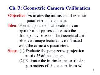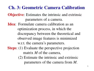
Geometric and Radiometric Camera Calibration
CSM4220. Geometric and Radiometric Camera Calibration. Shape From Stereo requires geometric knowledge of: Cameras’ extrinsic parameters, i.e. the geometric relationship between the two cameras.

Geometric and Radiometric Camera Calibration
E N D
Presentation Transcript
CSM4220 Geometric and RadiometricCamera Calibration • Shape From Stereo requires geometric knowledge of: • Cameras’ extrinsic parameters, i.e. the geometric relationship between the two cameras. • Camera intrinsic parameters, i.e. each camera’s internal geometry (e.g. Focal Length) and lens distortion effects. • Shape From Shading requires radiometric knowledge of: • Camera detector uniformity (e.g. Flat-field images) • Camera detector temperature noise (e.g. Dark frame images) • Camera detector bad pixels • Camera Digital Number (DN) to radiance transfer function 1
Camera Radiometric Calibration - 1 • All cameras require radiometric calibration, and this is most important for correct science image data interpretation. Basic radiometric calibration requires three types of image exposure: • Dark Frame – Typically a long exposure with no light being received by the camera detector (e.g. lens cap on). This is required to remove extraneous detector noise, and is very easy to perform for terrestrial applications. However, dark frames must be captured at those temperatures that will be experienced by the detector when capturing images. Example dark frame showing ‘hot’ pixels 2 CSM4220
Camera Radiometric Calibration - 2 • Bias Frame - Zero-length camera detector exposure. This is required to compensate for different pixel ‘start-up’ values (due to the bias offset applied to the A-D converter). The main issues here are that bias frames should also be captured at those temperatures that will be experienced by the detector, and to ensure that the camera detector software permits this type of exposure. However, they are not needed if the dark frames match the exposure time of the images from which they are to be subtracted, since dark frames contain bias information. 3 CSM4220
Camera Radiometric Calibration - 3 • Flat Field - Exposure of a uniform white surface. This is required to remove artefacts from 2D images that are caused by variations in the pixel-to-pixel sensitivity of the detector and/or by distortions in the optical path (e.g. dust on lens, vignetting, unequal pixel light sensitivity). This is harder to set up, and should be dark frame adjusted. The main problem is obtaining a white ‘surface’ that is truly uniform. In order to overcome this problem, an integrating sphere is used. Ideally a flat field image should be dark frame corrected to create a calibrated flat field image. 4 CSM4220
Camera Radiometric Calibration - 4 Raw image Calibrated flat field image derived from average of 4 × captured flat field images (minus dark frame) Flat field corrected image mean_of_calibrated_flat_field_image corrected_pixelx,y = (raw_pixelx,y – Dark_image_pixelx,y) × calibrated_flat_field_pixelx,y 5 CSM4220
Camera Radiometric Calibration - 5 • Cameras generate a Digital Number (DN) for each pixel. The camera detector (e.g. a CCD) measures a voltage for each pixel which represents the amount of light that the pixel has received. This voltage is converted to a DN using an analogue to digital converter (ADC). For a commercial off the shelf (COTS) 8-bit camera, then the pixel DN range is from 0 to 255. • For applications such as shape from shading, then the DN value for each pixel needs to be converted to a physical quantity called radiance. This is a radiometric quantity, and is useful because it indicates how much of the (light) power emitted by an emitting or reflecting surface will be received by an optical system looking at the surface from some angle of view. • The units of radiance are W/m2/sr. The steradian (sr) unit is the 3D ‘cousin’ to the 2D radians unit. If filters are used on the camera, for example, then spectral radiance is used and the units are: W/m2/sr/nm. • A transfer function from DN to radiance is required which may, or may not, have a linear relationship. 6 CSM4220
Camera Radiometric Calibration - 6 • The DN to radiance transfer function can be obtained via laboratory measurements, and one method is shown below. Spectral Irradiance (W/m2) at the receiving aperture Radius of receiving aperture Nominal distance between source and receiving apertures Radius of source aperture Spectral radiance at the source aperture measured using a spectrometer Spectral radiance at the receiving aperture Example transfer function Example camera images 7 CSM4220
Shape From Shading - 1 The Shape From Shading (SFS) problem is how to compute the 3D shape (e.g. height-map) of a surface from a single black and white image of the surface, i.e. an image that shows the brightness (radiance) of the surface under known illumination conditions. Diagram courtesy E. Prados and O. Faugeras 8 CSM4220
Shape From Shading - 2 In the 70’s Horn1 was the first to formulate the Shape From Shading problem, and to realise that it required finding the solution to a nonlinear first-order Partial Differential Equation (PDE) referred to as the brightness equation: I (x1, x2) = R (n (x1, x2)), where (x1, x2) are the coordinates of a point x in the image. R is the reflectance map, I the brightness image, and n is the surface normal vector of the point x. Many SFS methods assume that the surface has Lambertian reflectance properties. 1Horn, Berthold K.P., Shape from Shading: A Method for Obtaining the Shape of a Smooth Opaque Object from One View, PhD thesis, 1970, Department Electrical Engineering, MIT. 9 CSM4220
Shape From Shading - 3 For a Lambertian surface, then the reflectance map R is the cosine of the angle between the light vector L(x), and the normal vector n(x) to the surface (Lambert’s Law): Vector dot product n L R = cos(L,n) = · |L| |n| The apparent brightness of Lambertian surface to an observer is the same regardless of the observer’s angle of view. The surface represents an ideal diffusely reflecting surface. Note: most real surfaces are notLambertian (see BRDF link). 10 CSM4220
Shape From Shading - 4 Sun Light cos(θ1) < cos(θ2), therefore Slope A is greater than Slope B Observer Surface normal θ2 θ1 cos(0°) = 1 cos(90°) = 0 Slope A Slope B Lambertian surface 11 CSM4220
Shape From Shading - 5 There have been many algorithms developed to solve the Shape From Shading problem, see: Zhang et. al., Shape from Shading: A Survey, IEEE Trans. Pattern Analysis and Machine Intelligence, 21, 8, 690-706,1999. A recent (AU) solution, called the Large Deformation Optimisation Shape From Shading (LDO-SFS) algorithm, has been generated that shows good results with Mars HRSC images from the Mars Express orbiter, see: R. O’Hara, and D. Barnes, A new shape from shading technique with application to Mars Express HRSC images, ISPRS Journal of Photogrammetry and Remote Sensing, 67, 27-34, 2012. LDO-SFS can use different surface reflectance models e.g. Lambertian, or Oren-Nayar. 12 CSM4220
Shape From Shading: LDO-SFS Original single Martian surface (2D) image from HiRISE (MRO) Ortho-image rendered (3D) DEM views created using shape-from-shading 13 CSM4220
Shape From Shading: LDO-SFS Left image is the single 2D HRSC (H1022) image used as the input to the AU SFS algorithm. The right image is the 3D DEM data generated by the SFS algorithm. The DEM has been reverse lighting rendered (as compared to the left input image) to demonstrate the 3D nature of the data. Note that the 3D DEM has not been rendered with the H1022 ortho-image. 14 CSM4220
Shape From Shading: LDO-SFS DEM Visualisation and Slope Maps The left image is a topographic colour-coded image of the SFS generated DEM. Here the white coloured areas are the highest regions, and the dark blue coloured areas are the lowest regions. The right image shows a colour-coded slope map of the SFS DEM data. Green: ≥ 0°to < 10°, Blue: ≥ 10° to < 20°, and Red: ≥ 20°to < ∞°. 15 CSM4220
Shape From Shading: LDO-SFS Single input image Output image NOTE - SFS now with perspective projection 16 CSM4220
Shape From Shading: LDO-SFS Single input image Output image NOTE - SFS now with perspective projection 17 CSM4220
Stereo Vision (SV) versus Shape From Shading (SFS) • Both SV and SFS require accurate and precise calibration. • SFS requires accurate and precise knowledge of the lighting and observer vectors relative to the scene surface. • SV requires two images, SFS requires only one image. • SV provides absolute scene scale and dimensions. SFS has no concept of absolute scene scale and dimensions. • SV accuracy falls off with distance (remember D ∝1/d). SFS accuracy not dependent on scene distance. • SV works well when texture is present for disparity algorithm, e.g. good on rocks, but poor on sand dunes. SFS does not require texture, but does require that surface reflectance assumptions model reality (e.g. Oren-Nayar etc.). • SV good at modelling low-frequency scene structure, whereas SFS is good at modelling high-frequency scene structure. Solution: combine strengths of both methods. For an example see: Cryer, J.E, et. al., Integration of Shape From Shading and Stereo, Pattern Recognition, Vol. 28, No. 7, 1033-1043, 1995. 18 CSM4220