Ch. 3: Geometric Camera Calibration

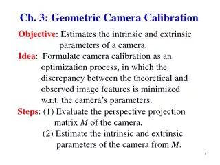
1. Ch. 3: Geometric Camera Calibration Objective: Estimates the intrinsic and extrinsic parameters of a camera. Idea: Formulate camera calibration as an optimization process, in which the discrepancy between the theoretical and observed image features is minimized w.r.t. the camera’s parameters. Steps: (1) Evaluate the perspective projection matrix M of the camera, (2) Estimate the intrinsic and extrinsic parameters of the camera from M.

2. 。 Perspective Projection (Imaging Process) where ideally, practically,

3. ○ Evaluate M Let Measure n pairs of corresponding image and scene points.

4. For each pair we obtain For all pairs,

5. In matrix form, where

6. Solve for x using optimization techniques

7. 3.1 Least-Squares Parameter Estimation Idea: Find the solution x by minimizing the squared deviation ( ) from theoretical (Ux) to observed (y) image features 3.1.1 Linear Least-Squares Methods ○ Consider a system of p linear equations in q unknowns:

8. In vector-matrix form, , where ,

9. ○ Consider the over-constrained case (p > q) • Find x that minimizes the error Let The normal equations : the pseudoinverse of U.

10. Homogenous systems: Two issues: (i) By equation , we obtain trivial solution (ii) If x is a solution, x is also a solution. To resolve the issues, impose 。 The least squares error solution of is the eigenvector of corresponding to the smallest eigenvalue.

11. 。 Find the least squares error solution by the method of Lagrange multipliers Error: Constraint Minimize where : Lagrange multiplier Let We obtain The solution x is an eigenvector of with eigenvalue

12. The associated error The least squares error solution to is the eigenvector of corresponding to the smallest eigenvalue. Example: Fit a line to a set of data points in the 2D space

13. Line equation: Let

14. The perpendicular distance from point to line is Error measure: Minimize E w.r.t. (a, b, d) Let

15. where 。Recall , whose squared error The solution of min w.r.t. n under constraint is the unit eigenvector with the minimum eigenvalue of

16. 3.1.2 Nonlinear Least-Squares Methods where

17. f(x): e.g., f(x): e.g.,

18. : the Jacobian of f where

19. 。Taylor expansion of around point f(x): f(x) :

20. Newton’s Method (Gradient Descent) • (i) Square Systems (p = q) • Idea: Given an initial x, find . . s.t. Since : nonsingular, When Let Repeat until f(x) stabilizes at some x • Drawbacks: i) Square system, ii) Nonsingular iii) Locally optimal.

21. Finding x s.t. Finding x s.t. F(x) = 0 (square system) : p by q matrix, f(x): p by 1, Since : q by 1

22. : q by q matrix where

31. (g) Proof: From

33. From and

35. ○ Degenerated Point Configurations e.g., points lie on a line or a plane, may cause failure of camera calibration. 3.3. Shape Distortions Types of distortions: (a) Tangential distortion (b) Radial distortion Barrel distortion, Pincushion distortion

36. Radial distortion: (a) Changes the distance between the image center and the image point (b) Does not affect the direction joining the image center and the image point d: actual distance : distorted distance : distortion function

37. Polynomial model: where : coefficients • FOV model: : distortion coefficient where • Logarithmic model, Fisheye model, • Radial model, Rational function model

38. 。 Consider Polynomial model Given an image point (u,v), determine its actual d

39. Determine the distortion function i.e., its coefficients

50. 3.5 Application: Mobile Robot Localization -- Calibrate a static camera for monitoring a robot