Camera Calibration
Camera Calibration. Camera calibration. Resectioning. Basic equations. minimize subject to constraint. Basic equations. minimal solution. P has 11 dof, 2 independent eq./points. 5½ correspondences needed (say 6). Over-determined solution. n 6 points.

Camera Calibration
E N D
Presentation Transcript
minimize subject to constraint Basic equations minimal solution P has 11 dof, 2 independent eq./points • 5½ correspondences needed (say 6) Over-determined solution n 6 points
Degenerate configurations • More complicate than 2D case (see Ch.21) • Camera and points on a twisted cubic • Points lie on plane and single line passing • through projection center No unique solution; camera solution moves arbitrarily along the twisted Cube or straight line.
Data normalization Less obvious (i) Simple, as before RMS distance from origin is √ 3 so that “average” point has coordinate mag of (1,1,1,1)T. Works when variation in depth of the points is relatively small, i.e. compact distribution of points (ii) Anisotropic scaling some points are close to camera, some at infinity; simple normalization doesn’t work.
Line correspondences Extend DLT to lines (back-project line lito plane ) For each 3D to 2D line correspondence: (2 independent eq.) X1 X2 X1 and X2 are points
Geometric error P Xi = Assumes no error in 3D point Xi e.g. accurately Machined calibration object; xi is measured point and has error
Gold Standard algorithm • Objective • Given n≥6 3D to 2D point correspondences {Xi↔xi’}, determine the Maximum Likelyhood Estimation of P • Algorithm • Linear solution: • Normalization: • DLT: form 2n x 12 matrix A by stacking correspondence Ap = 0 subj. • to ||p|| = 1 unit singular vector of A corresponding to smallest • singular value • Minimization of geometric error: using the linear estimate as a starting point minimize the geometric error: • Denormalization: ~ ~ ~ use Levenson Marquardt
Calibration example • Canny edge detection • Straight line fitting to the detected edges • Intersecting the lines to obtain the images corners • typically precision of xi <1/10 pixel • (HZ rule of thumb: 5n constraints for nunknowns 28 points = 56 constraints • for 11 unknowns DLT Gold standard
Errors in the world is closest point in space to Xi that maps exactly to xi Errors in the image and in the world Must augment set of parameters by including Mhanobolis distance w.r.t. known error covariance matrices for Each measurement xi and Xi
Restricted camera estimation • Find best fit that satisfies • skew s is zero • pixels are square • principal point is known • complete camera matrix K is known • Minimize geometric error • Impose constraint through parametrization • Assume square pixels and zero skew 9 parameters • Apply Levinson-Marquardt • Minimizing image only error f: 9 2n, • But minimizing 3D and 2D error, f: 3n+9 5n • 3D points must be included among the measurements • Minimization also includes estimation of the true position of 3D points
Minimizing Alg. Error. • assume map from parameters q P=K[R|-RC], i.e. p=g(q) • Parameters are principal point, size of square pixels and 6 for rotation and translation • minimize ||Ag(q)|| • A is 2n x 12; reduce A to a square 12x12 matrix independent of n such that for any vector p Mapping is from R9 R12
Restricted camera estimation • Initialization • Use general DLT to get an initial camera matrix • Clamp values to desired values, e.g. s=0, x= y • Use the remaining values as initial condition for iteration • Hopefully DLT answer close to “known” parameters and clamping doesn’t move things too much; Not always the case in practice clamping leads to large error and lack of convergence. • Alternative initialization • Use general DLT for all parameters • Impose soft constraints • Start with low values of weights and then gradually increase them as iterations go on.
Exterior orientation Calibrated camera, position and orientation unkown Pose estimation 6 dof 3 points minimal Can be shown that the resulting non linear equations have Four solutions in general
Restricted camera parameters; algebraic R9 R12 super fast Geometric: R9 R2n 2n = 396 in this case; super slow Same problem with no restriction on camera matrix Note: solutions are different!
Radial distortion short focal length long focal length; Distortion worse for short focal length
Correction of distortion x and y are the measured coordinates; Choice of the distortion function and center: xc and yc • Computing the parameters of the distortion function • Minimize with additional unknowns: i.e. estimate kappa, center and P • simultaneously • Straighten lines: determine L (r) so that images of straight scene lines • should be straight; then solve for P
K1 = 0.103689; k2 = .00487908; k3 = .0016894; k4 = .00841614 Xc = 321.87; yc = 241.18 ; original image: 640 x 480; periphery of image Moved by 30 pixels