Download

1 / 21
220 likes | 407 Vues
Parallel TSP with branch and bound. Presented by Akshay Patil Rose Mary George. Roadmap. Introduction Motivation Sequential TSP Parallel Algorithm Results References. Introduction. What is TSP?

E N D
Parallel TSP with branch and bound Presented by Akshay Patil Rose Mary George
Roadmap • Introduction • Motivation • Sequential TSP • Parallel Algorithm • Results • References
Introduction • What is TSP? • Given a list of cities and the distances between each pair of cities, find the shortest possible route that visits each city exactly once and returns to the original city.
Introduction • Problem Representation • Undirected weighted graph, such that the cities are graph vertices and paths are graph edges and a path's distance is the edge's weight.
Roadmap • Introduction • Motivation • Sequential TSP • Parallel Algorithm • Results • References
Motivation • Travelling salesperson problem with branch and bound is one of the algorithms which is difficult to parallelize. • Branch and bound technique can incorporate application specific heuristic techniques • One of the earliest applications of dynamic programming is the Held-Karp algorithm that solves the problem in O( n22n) • Greedy algorithm, may or may not obtain the optimal solution with O( n2 logn) complexity. • Parallel branch and bound optimization problems are large and computationally intensive. • Increasing availability of multicomputers, multiprocessors and network of workstations
Applications • TSP has several application even in its purest formulation such as : • Planning • Logistics • Manufacture of microchips • Genetics • UPS saves 3 million gallons of gasoline per year.
Roadmap • Introduction • Motivation • Sequential TSP • Parallel Algorithm • Results • References
Sequential TSP with branch and bound • Best_solution_node = null • Insert start city node into priority queue (Q) • While Q is not empty: • node = Q.top() // Node with least cost • If node.cost>= Best_solution_node.cost // Bound • continue • If node is solution better than Best_solution_node • Best_solution_node = node • Else • Explore children of node and insert in Q //Branch • Display best_solution_node
Sequential TSP with branch and bound noOfVertices = 5 Children Generated = (5-1 )! With No bounding
Sequential TSP with branch and bound noOfVertices = 5 Children Generated < (5-1 )! With bounding
Lower Bound Estimate • Cost of any node = path_cost + lower_bound_estimate • lower_bound_estimate = MST ( unvisitied cities, startcity, currentcity) • MST is calculated using Prim’s algorithm which takes O(n2) if implemented using adjacency matrix. • Why MST is a good estimate?
Roadmap • Introduction • Motivation • Sequential TSP • Parallel Algorithm • Results • References
Parallel Algorithm Datatype Creation for Solution Node • MPI_Datatypempinode; • MPI_Datatypetype[3] = {MPI_INT,MPI_INT,MPI_INT}; • MPI_Aintdisp[3]; • disp[0] = (int)&root.nvisited - (int)&root; • disp[1] = (int)&root.cost - (int)&root; • disp[2] = (int)&root.path[0] - (int)&root; • intblocklen[3] = { 1, 1, GRAPHSIZE }; • MPI_Type_create_struct(nodeAttributes,blocklen, disp, type, • &mpinode// Resulting datatype. • ); struct Node{ intnvisited; int cost; int path[GRAPHSIZE]; } // GRAPHSIZE = no.of.vertices
Parallel Algorithm • Send & Receive • At sender • MPI_Isend(&node, 1, mpinode,i,50,MPI_COMM_WORLD,&req); • node = variable of type Node • 1 = send 1 variable • Dataype = mpinode • At Receiver • MPI_Irecv(buffer, size, mpinode, MPI_ANY_SOURCE, 50, MPI_COMM_WORLD,&req); • MPI_Wait(&req, &status); • MPI_Get_count(&status, mpinode, &noOfNodesReceivedInBuffer);
Startup phase • Distribution of initial nodes to processors. • For noOfProcessors = 4 • Round 1 (start round = 1) • 0 generates children of start city, sends half to 1, keeps half in startupNodes • Round 2 (last round = log(noOfProcessors)) • 0 generates children nodes in startupNode, sends half to 2 • 1 generates children nodes in startupNode, sends half to 3
Roadmap • Introduction • Motivation • Sequential TSP • Parallel Algorithm • Results • References
Results For n = 12 For n = 12, all edge weights=10 except 1
Current State of the Art Algorithms • LKH(Lin-Kernighan heuristic), was used to solve the World TSP problem which uses data for all the cities in the world. • The best lower bound on the length of a tour for the World TSP is 7,512,218,268 • The tour of length 7,515,778,188 was found on October 25, 2011.
References • MPI Dynamic receive and Probe, http://www.mpitutorial.com/dynamic-receiving-with-mpi-probe-and-mpi-status/ • TSP Test Data, http://www.tsp.gatech.edu/data/ • World TSP, http://www.tsp.gatech.edu/world/index.html • LKH(Lin-Kernighan heuristic), http://www.akira.ruc.dk/~keld/research/LKH/ • Used to solved the World TSP problem