Download
1 / 47
470 likes | 668 Vues
PS, SSP, PSPI, FFD. KM. SSP. PSPI. FFD. z. 2. 2. k = k 1 – k. ~ k (1 – k + ..). x. x. z. k. 2. k. 2. 2. k. z. k. x. ik(x). z. P(x,z, w ) = P(x,0 , w ) e. PS, SSP, PSPI, FFD. 2. 2. 2. k = k 1 – k. k. k.

E N D
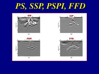
PS, SSP, PSPI, FFD KM SSP PSPI FFD
z 2 2 k = k 1 – k ~ k (1 – k + ..) x x z k 2 k 2 2 k z k x ik(x) z P(x,z,w) = P(x,0 ,w) e
PS, SSP, PSPI, FFD 2 2 2 k = k 1 – k k k ~ k (1 – .43k ) ~ k(1 – k ) z x x z z z k 2 k 2 2 2 k 1 2 ; k = k x k 2 k z ik(x) 1 -.5 z .2 P(x,z,w) = P(x,0 ,w) e -1 1 k x
SSP Migration 2 2 = k 1 – k k = k(x) 1 – k z - Dk x x z k(x) k 2 2 0 0 Thin lens ik(x) z P(x,z,w) = P(x,0 ,w) e
FFD Migration 2 2 = k 1 – k k = k(x) 1 – k z - Dk x x z k(x) k 2 2 0 0 Thin lens ik(x) z P(x,z,w) = P(x,0 ,w) e
FFD Migration 2 2 = k 1 – k k = k(x) 1 – k z - Dk x x z k(x) k 2 2 0 0 Thin lens ik(x) z P(x,z,w) = P(x,0 ,w) e
FFD Migration z ik(x) z P(x,z,w) = P(x,0 ,w) e
FFD Migration other term z ik(x) z P(x,z,w) = P(x,0 ,w) e
FFD Migration other term z PDE associated with other term Rearrange PDE ik(x) z P(x,z,w) = P(x,0 ,w) e
FFD Migration z Substitute FD approximations into above ik(x) z P(x,z,w) = P(x,0 ,w) e
FFD Migration z Substitute FD approximations into above ik(x) z P(x,z,w) = P(x,0 ,w) e
FFD Migration 2 2 = k 1 – k k = k(x) 1 – k z - Dk x x z k(x) k 2 2 0 0 Thin lens ik(x) z P(x,z,w) = P(x,0 ,w) e
Summary Cost: Accuracy: KM SSP PSPI FFD
Course Summary m(x)= a(g,s,x) G(g|x)d(g|x)G(x|s)dgds g,s,w d(g|x) = d(g|x) + d(x|g) G(g|x) = G(g|x) + G(g|x) Filter d(g|x) = d(g|x) G(g|x) = G(g|x) RTM Asymptotic G + Fresnel Zone 1-way G Asymptotic G KM Phase Shift Beam
Multisource Seismic Imaging vs CPU Speed vs Year 100000 10000 copper 1000 Aluminum VLIW Speed 100 Superscalar 10 RISC 1 1970 1980 1980 1990 2000 2010 2020 Year
OUTLINE Theory I Numerical Results Theory II
RTM Problem & Possible Soln. Problem: RTM computationally costly Solution: Multisource LSM RTM Preconditioning speeds up by factor 2-3 LSM reduces crosstalk 19 5
Ld +L d 1 2 2 1 = L d +L d + =[L +L ](d + d ) 1 2 1 2 1 1 2 2 d +d =[L +L ]m 1 2 1 2 mmig=LTd Multisource Migration: Multisource Least Squares Migration { { L d Forward Model: T T T T T T Crosstalk noise Standard migration
Orthogonal phase encoding s.t. <N* N >=0 1 2 = L d + L d =N*NL d +N*N L d + N*N L d + N*N L d =[NL +N L ](N d + Nd ) 1 2 2 1 1 2 1 1 2 1 2 2 2 2 2 2 2 1 1 1 1 1 1 2 2 1 1 2 Multisource Least Squares Phase-encoded Migration * * T T mmig Crosstalk noise T T T T If <N N > = d(i-j) i j Standard migration
2 2 2 (k) 2 [ N(t) ] [ N(t) ] N(t ) [ S(t) ] [S(t) +N(t) ] Key Assumption M M M M M k=1 k=1 k=1 k=1 k=1 Zero-mean white noise: <N(t)>=0; <N(t) N(t’) >=0 d(t) = Amplitude + M= Stack Number <N(t)> ~ 1 M (k) [ S(t) ] M 2 2 [ S(t) ] M 2 2 ~ ~ ~ SNR (k) (k) M s M vs M M
Multisource S/N Ratio L [d + d +.. ] d , d , …. d +d +…. L [d + d + … ] T T 2 1 2 1 2 2 1 1 # CSGs # geophones/CSG
Multisrc. Migration vs Standard Migration # geophones/CSG # CSGs MS MS MI vs MS M ~ ~ S-1 Iterative Multisrc. Migration vs Standard Migration # iterations vs
Ld +L d 1 2 2 1 Summary T T Time Statics 1. Multisource crosstalk term analyzed analytically 2. Crosstalk decreases with increasing w, randomness, dimension, iteration #, and decreasing depth Time+Amplitude Statics 3. Crosstalk decrease can now be tuned QM Statics 4. Some detailed analysis and testing needed to refine predictions.
OUTLINE Theory I Numerical Results Theory II
The Marmousi2 Model 0 Z k(m) 3 0 X (km) 16 The area in the white box is used for S/N calculation.
Conventional Source: KM vs LSM (50 iterations) 0 Z k(m) 3 0 X (km) 16 0 Z (km) 3 0 X (km) 16
200-source Supergather: KM vs LSM (300 its.) 0 Z k(m) 3 0 X (km) 16 0 Z (km) 3 0 X (km) 16
S/N = The S/N of MLSM image grows as the square root of the number of iterations. 7 S/N I 0 300 1 Number of Iterations
Multisource Technology • Fast Multisource Least Squares Phase Shift. • Multisource Waveform Inversion (Ge Zhan) • Theory of Crosstalk Noise (Schuster) 8
The True Model use constant velocity model with c = 2.67 km/s center frequency of source wavelet f = 20 Hz
Multi-source PSLSM • 645 receivers and 100 sources, equally spaced • 10 sets of sources, staggered; each set constitutes a supergather • 50 iterations of steepest descent
Single-source PSLSM • 645 receivers and 100 sources, equally spaced • 100 individual shots • 50 iterations of steepest descent
Multi-Source Waveform Inversion Strategy (Ge Zhan) 144 shot gathers Generate multisource field data with known time shift Initial velocity model Generate synthetic multisource data with known time shift from estimated velocity model Multisource deblurring filter Using multiscale, multisource CG to update the velocity model with regularization
3D SEG Overthrust Model(1089 CSGs) 15 km 3.5 km 15 km
Numerical Results Dynamic QMC Tomogram (99 CSGs/supergather) Static QMC Tomogram (99 CSGs/supergather) 3.5 km Dynamic Polarity Tomogram (1089 CSGs/supergather) 15 km
OUTLINE Theory I Numerical Results Theory II
Multisource Least Squares Migration Crosstalk term Time Statics Time+Amplitude Statics QM Statics 36
Summary Crosstalk term Time Statics 1. Multisource crosstalk term analyzed analytically 2. Crosstalk decreases with increasing w, randomness, dimension, and decreasing depth Time+Amplitude Statics 3. Crosstalk decrease can now be tuned QM Statics 4. Some detailed analysis and testing needed to refine predictions. 37
d +d =[L +L ]m 1 2 1 2 mmig=LTd Multisource Migration: Multisource Least Squares Migration { { L d Forward Model: Phase encoding Kirchhoff kernel Standard migration Crosstalk term 34
Multisource Least Squares Migration Crosstalk term 35
Multisource Least Squares Migration Crosstalk term Time Statics Time+Amplitude Statics QM Statics 36
Ld +L d 1 2 2 1 Crosstalk Term T T Time Statics Time+Amplitude Statics QM Statics
Summary Crosstalk term Time Statics 1. Multisource crosstalk term analyzed analytically 2. Crosstalk decreases with increasing w, randomness, dimension, and decreasing depth Time+Amplitude Statics 3. Crosstalk decrease can now be tuned QM Statics 4. Some detailed analysis and testing needed to refine predictions. 37
Multisource FWI Summary (We need faster migration algorithms & better velocity models) Stnd. FWI Multsrc. FWI IO 1 vs 1/20 Cost 1 vs 1/20 or better Sig/MultsSig ? Resolution dx 1 vs 1
2 2 (k) (k) (k) [ N(t ) ] N(t ) [ N(t ) ] Key Assumption n n n k=1 k=1 k=1 Zero-mean white noise: <N>=0; <N N >=0 i j <d(t)>= <S(t)> + <N(t)> Amplitude + n= Stack Number <N(t)> ~ n n 1/n 2 2 2 <N(t)> ~ <S(t)> ~ <N(t) > ~ <N(t) > ~ 2 2 1/n 1/n