Review
Review. As sample size increases, the distribution of sample means Becomes wider and more normally shaped Becomes narrower and more normally shaped Becomes wider and less normally shaped Becomes narrower and less normally shaped. Review.

Review
E N D
Presentation Transcript
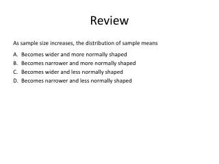
Review As sample size increases, the distribution of sample means • Becomes wider and more normally shaped • Becomes narrower and more normally shaped • Becomes wider and less normally shaped • Becomes narrower and less normally shaped
Review A population has a mean of µ = 10 and a standard deviation of s = 5. You plan to sample 100 people. What’s the expected value of your sample mean, M? • 0.5 • 1 • 5 • 10
Review A population has a mean of µ = 10 and a standard deviation of s = 5. You plan to sample 100 people. The expected (average) value of M is equal to µ, but M for any specific sample will be off, either too high or too low. How far from µ will the sample mean typically be? • 0.5 • 1 • 5 • 10
One-sample t-test 10/7
Hypothesis Test for Population Mean • Goal: Infer m from M • Null hypothesis (H0): m = m0 • Usually 0 • Sometimes another value, e.g. from larger population • Change scores • Memory improvement, weight loss, etc. • Sub-population within known, larger population • IQ of CU undergrads • Approach: • Determine likelihood function for M, using CLT • Compare actual sample mean to critical value
Likelihood Function for M • Probability distribution for M, according to H0 • Central Limit Theorem: • Mean equals population mean: mM = m0 • Standard deviation: • Shape: Normal p(M) Probability sM m0
Critical Value for M • Result that has 5% (a) chance of being exceeded, IF null hypothesis is true • Easier to find after standardizing p(M) • Convert distribution of sample means to z-scores: • Critical value for zM always the same • Just use qnorm() • Equals 1.64 for a = 5% p(M) p(zM) Probability Probability sM 1 a a m0 Mcrit zcrit 0
Example: IQ • Are CU undergrads smarter than population? • Sample size n = 100, sample mean M = 103 • Likelihood function • If no difference, what are probabilities of sample means? • Null hypothesis: m0 = 100 • CLT: • z-score: (103-100)/1.5 = 2 • mM = 100 • sM = s/√n = 15/10 = 1.5 zcrit M zM
Problem: Unknown Variance • Test statistic depends on population parameter • Can only depend on data or values assumed by H0 • Could include s in null hypothesis • H0: m = m0 & s = s0 • Usually no theoretical basis for choice of s0 • Cannot tell which assumption fails • Change test statistic • Replace population SD with sample SD • Depends only on data and m0 • . ?
t Statistic • Invented in 1908 by “Student” at Guinness brewery • . • Deviation of sample mean divided by estimated standard error • Depends only on data and m0 • Sampling distribution depends only on n
t Distribution • Sampling distribution of t statistic • Derived from ratio of Normal and (modified) c2 • Depends only on sample size • Degrees of freedom: df = n – 1 • Invariant with respect to m, s • Shaped like Normal, but with fatter tails • Reflects uncertainty in sample variance • Closer to Normal as n increases • Critical value decreasesas n increases
Steps of t-test 1. State clearly the two hypotheses 2. Determine null and alternative hypotheses • H0: m = m0 • H1: m ≠ m0 3. Compute the test statistic t from the data • . 4. Determine likelihood function for test statistic according to H0 • t distribution with n-1 degrees of freedom 5. Find critical value • R: qt(alpha,n-1,lower.tail=FALSE) 6. Compare actual result to critical value • t < tcrit: Retain null hypothesis, μ = μ0 • t > tcrit: Reject null hypothesis, μ ≠ μ0
Example: Rat Mazes • Measure maze time on and off drug • Difference score: Timedrug – Timeno drug • Data (seconds): 5, 6, -8, -3, 7, -1, 1, 2 • Sample mean: M = 1.0 • Sample standard deviation: s = 5.06 • Standard error: SE = s/√n = 5.06/2.83 = 1.79 • t = (M – m0)/SE = (1.0 – 0)/1.79 = .56 • Critical value: qnorm(.05,7,lower.tail=FALSE) = 1.89 • t does not exceed critical value • Cannot reject null hypothesis • Assume no effect of drug
Review You run a t-test and get a result of t = 7. What is your conclusion? • Reject the null hypothesis because t is bigger than expected by chance • Reject the null hypothesis because t is smaller than expected by chance • Keep the null hypothesis because t is bigger than expected by chance • Keep the null hypothesis because t is smaller than expected by chance
Review You run a t-test and get a result of t = 2. What does the value of 2 mean in this case? • The alternative hypothesis is twice as likely to be true as the null hypothesis • The sample mean is twice as far from µ0 as you would expect by chance • The population mean is likely within ±2 of the sample mean • Your chance of a Type I error will double if you reject the null hypothesis
Review Your null hypothesis predicts the population mean should be µ0 = 0. You measure 16 people and calculate statistics of M = 4 and s = 32. What is the value of your t statistic? • 2 • 0.5 • 0.25 • 4

