Download
1 / 66
660 likes | 860 Vues
Physics & Uses of Supernovae. IAG-LENAC XIII Advanced School of Astrophysics Abril 2006 – Foz do Iguazu. Plan of talk:. An introduction to Supernovae: Facts & Prejudices Type Ia Brightness Calibration: Refinements SN Cosmology Results 1: The accelerated Universe (~1998)

E N D
Physics & Uses of Supernovae IAG-LENAC XIII Advanced School of Astrophysics Abril 2006 – Foz do Iguazu
Plan of talk: • An introduction to Supernovae: Facts & Prejudices • Type Ia Brightness Calibration: Refinements • SN Cosmology • Results 1: The accelerated Universe (~1998) • SN Precision Cosmology • Results 2: The “Dark Energy”
Supernovae in History Observed since ancient times, as early as 2nd century, by Chinese Astronomers (called “Guest Stars”) Notable Examples in the Milky Way: • 185: (A.D.) The first SN on record • 1006: The brightest SN ever (like a 1/4 Moon) • 1054: The Crab Nebula, not recorded in Europe (?) • 1572: Tycho SN • 1604: Kepler SN • 1665 (approx): Cassioppeia A, not seen at all (?!)
Extragalactic Supernovae 1885: S Andromedae. A peculiar SN in Andromeda Galaxy 1920-1930: Some observed in sundry galaxies IMPORTANCE: Led to the separation of SNe from Novae • 1934: Baade & Zwicky wrote a very influential paper • They standardized the use of the name “Supernovae” • They suggested the exploding star mechanism • They concluded that many more would be found with a well designed survey
Zwicky & Baade (1934) in context Lev Landau proposed the concept of a neutron star, an object formed of nuclear matter and supported against collapse by “degeneracy” pressure in 1932. In 1934 this was very new. The source of power for stars was still unknown, and it was very bold to propose the connection of SNe with collapse of stellar cores to form neutron stars, still just a theoretical possibility.
Zwicky & Minkowski (1934-1944) Zwicky secured a newly designed Schmidt telescope and started the first systematic SN search. In the first five years of the survey he found 20 SNe. Minkowsky took spectra of the SNe. For the first 12 he found: • Broad wiggles resembling P Cygni profiles • A very repetitive pattern from SNe to SNe • A very regular evolution for all of them along time • A completely unknown set of lines (i.e. wiggles) Finally, SN # 13 showed Hydrogen lines
Type I & Type II (☺) • This coincidence led to: • Type I (no H) & Type II (H) • The need for at least TWO explosion mechanisms The second mechanism had to wait until 1964, when Fowler & Hoyle suggested the runaway thermonuclear reaction of degenerated C as the power source of Type Ia SNe. They also suggested the scenario: A white dwarf star near the Chandrasekhar limit accreting mass from a companion.
Type I: Model leads naturally to “No H” Implies association of progenitors with varied stellar populations. None of the VERY young. Theory of nuclear combustion is well known (microphysics). Nuclear combustion in gravitational confinement is not (macro). Type II: Model requires massive stars (more than ~8 Msun) Implies association of progenitors with young stellar populations Theory of gravitational core collapse rests on unknown physics This is true both at the micro and macro levels.
Type I: Model leads naturally to “No H” Implies association of progenitors with varied stellar populations. None of the VERY young. Theory of nuclear combustion is well known (microphysics). Nuclear combustion in gravitational confinement is not (macro). Implies Homogeneity ! Source of inhomogeneity (?) Type II: Model requires massive stars (more than ~8 Msun) Implies association of progenitors with young stellar populations Theory of gravitational core collapse rests on unknown physics This is true both at the micro and macro levels.
Type I: Model leads naturally to “No H” Implies association of progenitors with varied stellar populations. None of the VERY young. Theory of nuclear combustion is well known (microphysics). Nuclear combustion in gravitational confinement is not (macro). • Two possible (similar) scenarios: • Collapse of Fe degenerate cores • Collapse of Ne-O cores (~8 Msun) Type II: Model requires massive stars (more than ~8 Msun) Implies association of progenitors with young stellar populations Theory of gravitational core collapse rests on unknown physics This is true both at the micro and macro levels.
Theory: Three main branches • Explosion (Engine): Nuclear & Particle/High Energy Physics • Expansion (Shock): Nucleosynthesis & Hydrodynamics • Atmosphere: Radiative Transfer (γ-rays, e+, UVOIR) in a medium moving supersonically Some theoreticl “Hits:” Discovery of the delayed shock mechanism Discovery of the powering chain 56Ni → 56Co → 56Fe Development of the Sovolev Method Discovery of the “W7” combustion model Development of interacting binary evolution
Spectral “Lines” & Classification Chemical elements of the outermost layers leave the imprint of their low exitation transitions. BUT: Due to the large expansion velocity SN lines are more complex and difficult to interpret than those of starts with a static atmosphere.
SN Classification H / no H Type II Type I Tipe III, IV, and IV (Zwicky) Obsolete since the ~60s
SN Classification H / no H Type I Type Ia Type II He / no He Plateau Linear Type Ib Define the main observables which will be used for years: 1.- Spectra near maximum light 2.- Light curve shapes Note: Absolute brightness is not considered in classification CRITICAL: Realization that Type Ia was not a “clean” group
SN Classification Plateau H / no H Type I Type Ia Type II Some (?) Plateau He / no He Type IIn no Si II / Si II Type Ib Type Ic SN 87K SN 93J Lineal Differences in Light Curves Problem: Number of core-collapse SNe imply more massive Stars than are currently available to produce progenitors. Problem: Type Ic is just “absence of evidence” (i.e. nothing)
Binary evolution & Transition SNe Two different Scenarios: Single and Coupled (binary) evolution More massive star evolves.
Binary Evolution & Transition SNe Inner structure will be similar even though outer layers will differ Core going to collapse is very similar, but external layers are very different
Binary Evolution & Transition SNe Generally star 2 will survive the explosion If star 2 also goes to explosion, a binary pulsar may result.
SN Classification Plateau H / no H Type I Type Ia Type II Some (?) Plateau He / no He Type IIn no Si II / Si II Type Ib Type Ic Type IIb Lineal Differences in Light Curves Gravitational collapse with Angular Momentum: GRB→Hypernovae
Spectroscopic Signs: SN 2003dh MMT (Stanek et al) VLT (Hjorth et al)
Jet break Photometric signs: SN 2003dh
SN Classification Plateau H / no H Type I Type Ia Type II Some (?) Plateau He / no He Type IIn no Si II / Si II Type Ib Type Ic Type IIb Lineal Differences in Light Curves Gravitational collapse with Angular Momentum: GRB→Hypernovae
In the meantime: The world of SN Ia was getting more homogeneous… or was it?
Type Ia SN Light Curves (version 70s) ~2.5 mag decay in ~30 days after maximum Fairly uniform light curves with. > 0.5 mag (at maximum) 38 SNe de tipo I (Barbon, Ciatti, & Rosino, 1973, AAp , 25, 241)
Type Ia SN Light Curves (version 70s) ~3.0 mag decay in ~30 days after maximum. 11 Type I SNe (Barbon, Ciatti, & Rosino, 1973, AAp , 25, 241)
Type Ia SN Light Curves (version 70s) ~2.0 mag decay in ~30 days after maximum. 27 Type I SNe (Barbon, Ciatti, & Rosino, 1973, AAp , 25, 241)
Type Ia SN Light Curves (version 90s) All of then decay differently!
Refinement of SNe Ia as Distance indicators Sandage and Tammann 1993 Hamuy et al. 1996 Kowal, 1968 SNe I are fair candles with ~1 mag SNe Ia are outstanding, ~ 0.2 mag, SNe Ia are pretty good, ~ 0.5 mag,
MB Light and Color Curve Calibrations Detailed empirical, prescriptions for measuring luminosity, reddening, distance, and uncertainty. Days after maximum Methods: Phillips 1993, 1999, Hamuy et al 1996; MLCS: Riess, Press, Kirshner 1995 1996, Riess et al 1998, Jha, Riess, Kirshner 2002; “stretch”: Perlmutter et al 1997, 1999
Hence: Type Ia SNe are precise standard(izable) candles s~0.11mag Prieto et. al. (2005) Krisciunas et. al. (2003)
Strong Impact on Between 1993 and 1999, Type Ia SNe become an almost ideal distance indicator for cosmologicaly relevant distances. Riess et al, 1997
The Cosmological Framework • Observations • The Universe is Expanding • CMB => Hot Big Bang • Theory & Hypothesis • General Relativity Principles (corroborated, so far, by observations) • Universe is homogeneous & isotropic on large scales. Friedman Equation (Equation of Motion of the Universe) (Dark) Matter (Dark) Energy (Cosmological Constant?) Geometry (Curvature)
Expansion History of the Universe Cosmological parameters imply destiny of Universe Redshift Distance But destiny is written in past expansion history (Hubble Diagram)
Luminosity Distances Cosmological Constant Curvature Mass The relation DL vs.z carries Ωk, ΩM and ΩΛas parameters.
Linear part of the HD, just kinematics. Non linear part of the HR (dynamics)
Differences are measurable! (with good distance estimators)
Hubble Diagram as a Cosmological Test ΩM=0, ΩΛ=0 ΩM=0.3, ΩΛ=0.7 ΩM=0.3, ΩΛ=0 ΩM=1, ΩΛ=0 Combining Theoretical DLwith real observations, build Ψ2 statistics, get probability of Ψ2 and confidence regions.
1998 Result: Acceleration! (HZSS) 85 local SNe 13 distant SNe 1 very distant SN (Riess et al. 1998)
Year 2005: Confirmation (HZSS) 85 local SNe (Clocchiatti et al. 2005) 29 distant SNe 18 verydistant SNe
Year 2005: All SN Sample 85 local SNe (Riess et al.) 56 distant SNe 36 verydistant SNe
Year 2005: SNe + Independent ΩM “Concordance” Universe ΩM~0.30 ΩΛ~0.70
In short: It DOES look like we will have to live with acceleration… But: Do we REALLY have to live with ΩΛ?