Download
1 / 28
280 likes | 415 Vues
DSCI 5340: Predictive Modeling and Business Forecasting Spring 2013 – Dr. Nick Evangelopoulos. Lecture 6: Box-Jenkins Models (Ch. 9). Material based on: Bowerman-O’Connell-Koehler, Brooks/Cole. Homework in Textbook. Page 398 Ex 8.1, Ex 8.2 parts a and b Ex 8.6 parts a and b Ex 8.11.

E N D
DSCI 5340: Predictive Modeling and Business ForecastingSpring 2013 – Dr. Nick Evangelopoulos Lecture 6: Box-Jenkins Models (Ch. 9) Material based on: Bowerman-O’Connell-Koehler, Brooks/Cole
Homework in Textbook Page 398 Ex 8.1, Ex 8.2 parts a and b Ex 8.6 parts a and b Ex 8.11
Exercise 8.1 Page 398 Part a. How do we calculate this number?
Exercise 8.1 Page 398 Part b. How do we calculate this number? Note that smoothed estimate at time period 3 is Forecast for time period 4.
Exercise 8.1 Page 398 Part c. How do we calculate this number?
Exercise 8.1 Page 398 Part d. How do we calculate this number? Note that smoothed estimate at time period 3 is Forecast for time period 4.
Ex. 8.11, page 399 First Get Regression Estimates for initial values for l0 and b0.
Ex. 8.11, page 399 Get Seasonal Estimates
Ex. 8.11, page 399 Get Smoothed Estimates & Forecasts Note: to get ssquare, subtract 3 degrees of freedom!
Ex. 8.11, page 399 Drag Formulas for complete table
Chapter 9 Box-Jenkins Methodology • This is a method for estimating ARIMA models, based on the ACF and PACF as a means of determining the stationarity of the variable in question and the lag lengths of the ARIMA model. • Although the ACF and PACF methods for determining the lag length in an ARIMA model are commonly used, there are other methods termed information criteria which can also be used (covered later)
Box-Jenkins • The Box-Jenkins approach typically comprises four parts: • Identification of the model • Estimation, usually OLS • Diagnostic checking (mostly for autocorrelation) • Forecasting
Elements of Box-Jenkins models • Box-Jenkins models are non-seasonal • Classical Box-Jenkins models describe stationary time series data • Nonstationary time series data can be transformed to stationary through differencing • ACF and PACF (SAC and SPAC) plots can be used to tentatively determine stationarity
Parsimonious Model • The aim of this type of modeling is to produce a model that is parsimonious, or as small as possible, while passing the diagnostic checks. • A parsimonious model is desirable because including irrelevant lags in the model increases the coefficient standard errors and therefore reduces the t-statistics. • Models that incorporate large numbers of lags, tend not to forecast well, as they fit data specific features, explaining much of the noise or random features in the data.
ARIMA (Box-Jenkins) Models • AutoRegressive Integrative Moving Average • Autoregressive – future values depend on previous values of the data • Moving average – future values depend on previous values of the errors • Integrated – refers to differencing the data
Stationary Models • Stationarity is defined as the property of a time series to have statistical properties (mean, variance) that are constant over time. • Non-stationary time series can (often) be transformed to stationary by taking the first (or second) differences. • This is the “integration” (the “I”) part in ARIMA
A first differencing example Non-stationary (notice the mean change) Stationary (the mean is now constant)
How to Determine if a Time Series is Stationary? SAC = Sample Auto-Correlation function (aka ACF)
ACF and PACF Printout of Autocorrelation Function (ACF) and Partial Autocorrelation Function (PACF)
Next lecture: AR and MA models Nonseasonal autoregressive model of order 1: Nonseasonal moving average model of order 1:
Homework in Textbook Page 438 Ex 9.2, Ex 9.3, Ex 9.4