Operations Research Modeling Toolset
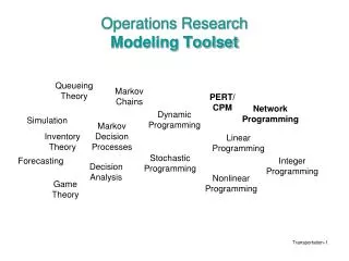
Operations Research Modeling Toolset Queueing Theory Markov Chains PERT/ CPM Network Programming Dynamic Programming Simulation Markov Decision Processes Inventory Theory Linear Programming Stochastic Programming Forecasting Integer Programming Decision Analysis

Operations Research Modeling Toolset
E N D
Presentation Transcript
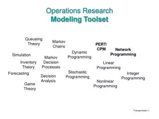
Operations Research Modeling Toolset Queueing Theory Markov Chains PERT/ CPM Network Programming Dynamic Programming Simulation Markov Decision Processes Inventory Theory Linear Programming Stochastic Programming Forecasting Integer Programming Decision Analysis Nonlinear Programming Game Theory
Network Problems • Linear programming has a wide variety of applications • Network problems • Special types of linear programs • Particular structure involving networks • Ultimately, a network problem can be represented as a linear programming model • However the resulting A matrix is very sparse, and involves only zeroes and ones • This structure of the A matrix led to the development of specialized algorithms to solve network problems
Types of Network Problems • Shortest Path Special case: Project Management with PERT/CPM • Minimum Spanning Tree • Maximum Flow/Minimum Cut • Minimum Cost Flow Special case: Transportation and Assignment Problems • Set Covering/Partitioning • Traveling Salesperson • Facility Location and many more
The Transportation Problem • The problem of finding the minimum-cost distribution of a given commodity from a group of supply centers (sources) i=1,…,mto a group of receiving centers (destinations) j=1,…,n • Each source has a certain supply (si) • Each destination has a certain demand (dj) • The cost of shipping from a source to a destination is directly proportional to the number of units shipped
Simple Network Representation Sources Destinations 1 Supply s1 1 Demand d1 Supply s2 2 2 Demand d2 … … xij n Demand dn Supply sm m Costs cij
Example: P&T Co. • Produces canned peas at three canneries Bellingham, WA, Eugene, OR, and Albert Lea, MN • Ships by truck to four warehouses Sacramento, CA, Salt Lake City, UT, Rapid City, SD, and Albuquerque, NM • Estimates of shipping costs, production capacities and demands for the upcoming season is given • The management needs to make a plan on the least costly shipments to meet demand
Example: P&T Co. Map 1 2 3 3 2 1 4
Example: P&T Co. Data Shipping cost per truckload
Example: P&T Co. • Network representation
Example: P&T Co. • Linear programming formulation Let xij denote… Minimize subject to
Feasible Solutions • A transportation problem will have feasible solutions if and only if • How to deal with cases when the equation doesn’t hold?
Integer Solutions Property: Unimodularity • Unimodularity relates to the properties of the A matrix(determinants of the submatrices, beyond scope) • Transportation problems are unimodular, so we get the integers solutions property: For transportation problems, when every si and dj have an integer value, every BFS is integer valued. • Most network problems also have this property.
Transportation Simplex Method • Since any transportation problem can be formulated as an LP, we can use the simplex method to find an optimal solution • Because of the special structure of a transportation LP, the iterations of the simplex method have a very special form • The transportation simplex method is nothing but the original simplex method, but it streamlines the iterations given this special form
Transportation Simplex Method Initialization (Find initial CPF solution) Is the current CPF solution optimal? Yes Stop No Move to a better adjacent CPF solution
Prototype Problem • Holiday shipments of iPods to distribution centers • Production at 3 facilities, • A, supply 200k • B, supply 350k • C, supply 150k • Distribute to 4 centers, • N, demand 100k • S, demand 140k • E, demand 300k • W, demand 250k • Total demand vs. total supply
Finding an Initial BFS • The transportation simplex starts with an initial basic feasible solution (as does regular simplex) • There are alternative ways to find an initial BFS, most common are • The Northwest corner rule • Vogel’s method • Russell’s method (beyond scope)
The Northwest Corner Rule • Begin by selecting x11, let x11 = min{ s1, d1 } • Thereafter, if xij was the last basic variable selected, • Select xi(j+1) if source i has any supply left • Otherwise, select x(i+1)j
The Northwest Corner Rule Z = 10770
Vogel’s Method • For each row and column, calculate its difference: = (Second smallest cij in row/col) - (Smallest cij in row/col) • For the row/col with the largest difference, select entry with minimum cij as basic • Eliminate any row/col with no supply/demand left from further steps • Repeat until BFS found
Vogel’s Method (3): update supply, demand and differences 90
Vogel’s Method (5): update supply, demand and differences 100 90
Vogel’s Method (7): update supply, demand and differences 100 50 90
Vogel’s Method (8): select xAS as basic variable 140 100 50 90
Vogel’s Method (9): update supply, demand and differences 140 100 50 90
Vogel’s Method (10): select xAW as basic variable 140 60 100 50 90
Vogel’s Method (11): update supply, demand and differences 140 60 100 50 90
Vogel’s Method (12): select xBW and xBE as basic variables 140 60 210 140 100 50 90 Z = 10330
Optimality Test • In the regular simplex method, we needed to check the row-0 coefficients of each nonbasic variable to check optimality and we have an optimal solution if all are 0 • There is an efficient way to find these row-0 coefficients for a given BFS to a transportation problem: • Given the basic variables, calculate values of dual variables • ui associated with each source • vj associated with each destination using cij – ui – vj = 0 for xij basic, or ui + vj = cij (let ui = 0 for row i with the largest number of basic variables) • Row-0 coefficients can be found from c’ij=cij-ui-vj for xij nonbasic
Optimality Test (1) 60 140 210 140 100 50 90
Optimality Test (2) • Calculate ui, vj using cij – ui – vj = 0 for xij basic (let ui = 0 for row i with the largest number of basic variables) 60 140 210 140 100 50 90
Optimality Test (3) • Calculate c’ij=cij-ui-vj for xij nonbasic 60 140 140 210 50 100 90
Optimal Solution Sources Destinations N Demand = 100 A 140 Supply = 200 60 S Demand = 140 210 Supply = 350 B 140 E Demand = 300 (shortage of 90) 100 Supply = 150 C 50 W Demand = 250 Cost Z = 10330
An Iteration • Find the entering basic variable • Select the variable with the largest negative c’ij • Find the leaving basic variable • Determine the chain reaction that would result from increasing the value of the entering variable from zero • The leaving variable will be the first variable to reach zero because of this chain reaction
Initial Solution Obtained by the Northwest Corner Rule 100 100 40 300 10 150 90
100 100 - + 40 300 10 150 + - 90 ? Iteration 1
End of Iteration 1 100 100 40 210 100 150 90
Optimality Test 100 100 40 210 100 150 90
Iteration 2 + - 100 100 + - 210 100 40 ? 150 90
End of Iteration 2 140 60 40 210 100 150 90
Optimality Test 140 60 40 210 100 150 90 Z = 10330
Optimal Solution Sources Destinations N Demand = 100 60 A Supply = 200 140 S Demand = 140 40 Supply = 350 B 210 E Demand = 300 (shortage of 90) 100 Supply = 150 C 150 W Demand = 250 Cost Z = 10330
The Assignment Problem • The problem of finding the minimum-costly assignment of a set of tasks (i=1,…,m) to a set of agents (j=1,…,n) • Each task should be performed by one agent • Each agent should perform one task • A cost cij associated with each assignment • We should have m=n (if not…?) • A special type of linear programming problem, and • A special type of transportation problem,with si=dj= ?