Download
1 / 13
130 likes | 374 Vues
Computational Nanophotonics -- S. K. Gray. Computational Nanophotonics Stephen K. Gray Chemistry Division Argonne National Laboratory Argonne, IL 60439 gray@tcg.anl.gov Tel: 630-252-3594. Motivation. surface-plasmon resonance in Au nanoparticles.

E N D
Computational Nanophotonics Stephen K. GrayChemistry DivisionArgonne National LaboratoryArgonne, IL 60439gray@tcg.anl.govTel: 630-252-3594
Motivation surface-plasmon resonance in Au nanoparticles • Wish to control light or electromagnetic energy in nano-sized optical devices • Problem: optical light has wavelength >> 1nm • Possible Solution - use near-field coupling of light with surface plasmons of metal nanoparticles => arrays of metal nanoparticles become photonic devices => steady or pulsed modes of illumination
Excitation Transfer in Nanophotonics Want Simulations to Guide Experiment • arrays of metal nanoparticles + substrate represented by spatially varying dielectric constant • discretized fields E and H on 3D grids • finite difference solution to Maxwell’s (curl) equations for time and spatial dependence of E and H fields
Finite Difference Time Domain (FDTD) Method Maxwell’s PDEs , outside nanoparticle: inside nanoparticle ∂E(x,t)/∂t = x H(x,t)/e(x) ∂E(x,t)/∂t = [ x H(x,t) - J(x,t)]/e∞ ∂H(x,t)/∂t = - x E(x,t)/µo ∂H(x,t)/∂t = - x E(x,t)/µo ∂J(x,t)/∂t = eowp2E(x,t)/µo -nJ(x,t) are discretized in space and time : in general, 6 or more components are represented on a 3D spatial grid and propagated in discrete time steps
FDTD Basics : Yee Algorithm based on staggered space and time grids Space : • Each E component surrounded by 4 H components • Each H component surrounded by 4 E components
Current ANL Calculations • 2D uniform grids (2000 x 2000) over 10000 time steps • Silver “nanowire” (nanoscale radius infinite cylinder) arrays considered • Variety of array configurations examined
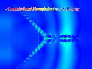
Example: pulse of vertically polarized, 400 nm light shows 100 nm scale localization when passing (left to right) through a funnel configuration of 30 nm diameter silver nanowires[S. K. Gray and T. Kupka, Phys. Rev. B, submitted (2003).] 600 nm 0 0 600 nm
Future Work Includes : • 3D Extensions for arbitrary shapes • The FD algorithm parallelization
Some Useful References : Quinten et al., Optics Letters 23, 1331 (1998) Maier et al., Advanced Materials 13, 1501 (2001) Maier et al., Appl. Phys. Lett. 81, 1714 (2002) Krenn et al., Europhys. Lett. 60, 663 (2002) Kottmann and Martin, Optics Express 12, 655 (2001)