Slow Servo Loops; Beam Phase Loops: Basic loop with differentiators;

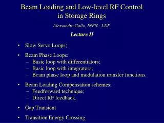
1. Beam Loading and Low-level RF Control in Storage Rings Alessandro Gallo, INFN - LNF Lecture II • Slow Servo Loops; • Beam Phase Loops: • Basic loop with differentiators; • Basic loop with integrators; • Beam phase loop and modulation transfer functions. • Beam Loading Compensation schemes: • Feedforward technique; • Direct RF feedback. • Gap Transient • Transition Energy Crossing

2. Slow servo loops

3. Beam For little cavity detuning (QLd << 1) the cavity response to an amplitude modulated signal is a single pole low-pass: AMPLITUDE LOOP The automatic regulation of the generator output level can be obtained by implementing amplitude loops. These are feedback systems which detect and correct variations of the level of the cavity voltage. If the power amplifier is not fully saturated, the regulation can be obtained by controlling the RF level of the amplifier driving signal. If the amplifier is saturated, the feedback has to act directly on the high voltage that sets the level of the saturated output power. Referring to the reported model, the loop transfer function can be written in the form:

4. Amplitude loops may have bandwidths ranging from few Hz to 1 MHz. Sometimes it is useful to have large residual loop gain at line frequencies to correct spurious modulation introduced by the power stages. The gain and bandwidth can be tailored by properly designing the error amplifier transfer function G(s). For instance, if the cavity single-pole model is adequate, high loop gains in the low frequency region are obtainable by implementing an integrator providing a zero for compensating the cavity pole. AMPLITUDE LOOP In heavy beam loading regime the cavity detuning is likely to be as large as the cavity bandwidth or even more, so that the single pole model for the cavity amplitude response is inappropriate. The completed Pedersen model applies in this case, involving cross-modulation blocks. The low frequency gain can be boosted by properly treating the error signal. However, the coupling between the various RF servo loops induced by the large cavity detuning may result in a global instability of the beam-cavity system. To avoid it, gain and bandwidth of individual loops have to be reduced.

5. Beam PHASE LOOP The cavity RF phase (or the power station RF phase) can be locked to the reference RF clock by another dedicated servo loop. The need for a phase loop is not strictly related to beam loading effects but more to ensure synchronization between different RF cavi-ties or between RF voltage and other sub-systems of the accelerator (such as injection system, beam feedback systems, ...). The phase is locked to the reference by measuring the relative phase deviation by means of a phase detector and applying a continuous correction through a phase shifter. For loopgain and bandwidth the same considerations expressed in the amplitude loop case hold.

6. Beamphase loops

7. Ideally, if the cavity modulation were exactly proportional to the time derivative of the beam phase we would get: making a frictional term appearing in the synchrotron equation. Beam Phase Loop The beam phase loops are feedback systems aimed at adding a damping (frictional) term in the synchrotron equation for the beam center-of-mass coherent motion. In the basic scheme the phase of the beam is detected and, after a manipulation to introduce a 90° phase shift at the synchrotron frequency, is applied back to the cavity.

8. The closed loop transfer function will have poles at:  1 Provided that wd <0 (negative feedback), the pole pair has a negative real part. A damping constant ad is added, given by:  0 while critical damping is achievable under the condition: Beam Phase Loop: Pure Differentiator A pure differentiator in the Laplace s-domain has a transfer funtion of the type G(s)=s/wd. If beam loading effects can be neglected, the open loop transfer function H(s) and the characteristic equation have the form: The gain of a pure differentiator circuit grows linearly with frequency, which is not a realistic behaviour for any physical system.

9. leading to the characteristic equation: By applying the Routh-Horwitz criterion, the zeros have negative real part if: Beam Phase Loop : Real Differentiator A real differentiator can be obtained by using the low frequency portion of the transfer function of a simple band-pass filter. In this case the loop amplifier has a transfer funtion of the type:

10. Real integrator, to be discussed later For real differentiators there is a limit on the maximum achievable loop gain in stable conditions. If w2 >> w1 this limit is given by: Beam Phase Loop : Real Differentiator The solutions have the form: It may be shown that in this case, even at the maximum gain, critical damping can not be reached. Beam phase loops based on real differentiator have been demonstrated to be effective in cases where limited extra-damping is needed. By tayloring the bandpass limits w1 , w2the loop repsonse at the revolution frequency can be reduced to avoid excitation of coupled bunch modes different from the barycentre one. Loop gain has also to be reduced if a the beam quadrupole resonance at 2ws is excited.

11. leading to the characteristic equation: By applying the Routh-Horwitz criterion, the zeros have negative real part if: Beam Phase Loop : Real Integrator To get damping from a beam phase loop the loop amplifier must provide 90° of phase rotation at ws. If a pure delay is used the results are similar to those obtained with differentiator. An alternative way of generating the 90° phase shift is to implement a real integrator, i.e. a LPF with the synchrotron frequency placed on the falling edge. The transfer function is: The case of a pure integrator G(s)=wi/s can be treated by considering G0=w1/wi, wi 0 and the system results to be unstable. In the real integrator case the range of acceptable gain is limited, while at the limit G0=1 one of the zeros is s=0 , which means that the closed loop system has a peaking response at low frequency. This limitation can be circumvented by AC coupling the loop (one or more zeros at s=0 in G(s)). With one zero we get back to the bandpass shape of G(s).

12. so that a double zero in the origin appears. If we consider a pure integrator transfer function G(s)=wi/s we obtain the characteristic equation: which is inconditionally stable for wi>0, and the damping constant ai=wi/2isindependent onws. Similar results (inconditioned stability, damping almost independent on ws) are found by if real integrator or real double integrator transfer functions are considered: Beam Phase Loop: Integrator over the beam-to-cavity phase Another way of obtaining AC coupling to implement an integrator loop amplifier is to feedback the beam-to-cavity phase. The open loop gain H(s) in this case results to be: All these schemes are in principle well performing but suffer of a common drawback. The loop is AC because of the B(s)-1 transfer function, but the branch from the phase detector PD to the phase shifter PS (including the loop amplifier) may have large DC gain. Any DC offset or drift from the PD would saturate either the loop amplifier or the PS, also producing unnecessary change of the cavity driving phase.

13. The real integrator transfer function can be recovered by using a Voltage Controlled Oscillator (VCO) AC coupled to the loop amplifier. The VCO can be considered as a phase shifter with infinite dynamics, adding apoleats=0(frequencytophase conversion). The VCO pole and the AC loop amplifier zero cancel out, so that: Beam Phase Loop: Integrator over the beam-to-cavity phase To avoid DC driving of the phase shifter, an AC coupled loop amplifier has to be implemented. The loop amplifier is a BPF acting as an integrator for frequencies located on the folling edge of the frequency response. In proton synchrotron the VCO may be DC driven by a proper signal to control the radial position of the bunches even during acceleration (revolution frequency, beam energy and radial position in a dispersive monitor are mutually proportional in this case, except in the vicinity of the transition energy). The beam phase loop does not interfere with low frequency regulations and provides damping of the coherent synchrotron motion.

14. Beam Phase Loop: DC coupled VCO with radial loop The DC coupling to the VCO can be restored if an additional loop correcting the DC set of the VCO frequency is implemented. If a “flat response” loop amplifier G(s) would be DC coupled to the VCO, any disturbance at the phase detector Dfn would produce a beam frequency deviation Dfb given by: Any phase offset disturbance drives the beam to a staedy frequency deviation. To avoid this effect the VCO can be feedback controlled by another DC loop looking at the radial position of the beam in a dispersive monitor (which is proportional to both the beam energy and the revolution frequency). Once this additional loop is set up we have:

15. Beam Phase Loop: DC coupled VCO with radial loop The radial loop compresses the residual beam frequency deviation Dfb by a factor Gf. Looking at the roots of the characteristic equation we have in this case: that holds under the assumptions |Gf |>>1 and wi2 >>ws2|Gf |. If Gf < 0, the system is stable with one large negative root strongly damping the coherent synchrotron motion, and a second weaker root damping the slow motion coming from low frequency disturbances. If the time constant associated to the second root is much longer that the synchrotron period, i.e. : the beam follows adiabatically the motion induced by the slow disturbances. The DC coupled VCO together with radial loop has been widely used in proton synchrotron. This set-up has shown good performances in strongly damping the coherent motion (which can not be even measured) and controlling the beam radial position.

16. If we consider a pure integrator loop amplifier G(s)=wi/s and a synchronous phase fs=± p/2 (to account for the 2 cases sgn(h)=± 1), the characteristic equation is: leading to the stability conditions: Beam Phase Loop Analysis with Modulation Transfer Functions We have so far analyzed beam phase loops neglecting the modulation transfer functions, which have to be included whenever beam loading effects are relevant. Referring to the complete block diagram aside, the open loop transfer H(s) function is given by:

17. Beam Phase Loop Analysis with Modulation Transfer Functions The presence of the beam phase loop enlarge the Robinson 1st stability limits since also a region with fz<0 (fz>0 for h<0 ) becomes accessible. This is because the strong loop damping of the coherent motion overrides the Robinson antidamping. The Robinson 2nd limit is unaffected since it is a DC instability, and the beam phase loop has no DC gain in the considered configuration. However, realistic models of RF systems are much more complicated since other loops have to be included (at least tuning and amplitude loops) and real transfer functions contain delay terms together with roll-off frequencies which are intrinsic of the used devices. Realistic cases can be better treated numerically. Numerical approach shows that the presence of many loops decreses the stability region of the system, especially if the loop bandwidths are comparable with (or larger than) the cavity half-bandwidth s. In the oversimplyfied scenario of pure integrator loop transfer functions, fs=± p/2, fg=0,s>> wi and B(s)=0, F. Pedersen has derived the following stability criterion: where wp, wa, wt are the integrator constants of the phase, amplitude and tuning loops. If a too low limit on Y results, the beam loading effects have to be cured with dedicated techniques to cancel or limit the perturbation induced by the beam signal in the RF system.

18. Feedforward Technique

19. A very elegant way to compensate the beam loading effects is the so called “feedforward”. If a beam signal sample is injected back in the RF driving path with a proper amplitude and phase, it is possible to generate through the RF power source a contribution to the cavity voltage equal and opposite to that induced by the beam. Ideally, looking at the system from reference clock path, no beam induced effects are visible. The RF generator current in the model can be split in 2 contributions, coming from drive and feedback signals. If the feedback is properly set, the current If and Ib cancel out, so that the total current It exciting the cavity is equal to the current Id generated by the drive signal alone. Beam Loading Compensation: The Feedforward Technique

20. p Cavity Beam + p p Cavity Beam p + Drive + p p Drive + a a a p + a a + a Feedforward a “Plain” modulation functions (no vector projection) Beam Loading Compensation: The Feedforward Technique It has to be pointed out that the “feedforward” can not change the static beam loading effects. The power delivered by the generator is just the same, and so it is the beam induced voltage and the need for a cavity detuning proportional to the stored current. What the feedforward does change is the dynamics of the beam loading, leading to a substantial simplification of the Pedersen representation of the system. The feedback signal and the beam have the same modulation transfer functions to the cavity voltage (the 2 phasors have the same phase). So the feedback cancel out the beam to cavity modulation terms in the Pedersen model.

21. Beam Loading Compensation: The Feedforward Technique • Feedforward technique has been successfully implemented in some “hystorical” proton synchrotron machines such as the CERN PS and ISIS. • However, in spite to the great elegance and conceptual simplicity, the compensation scheme is quite critical for a number of reasons, namely: • non linearity and drifts of the characteristics of the RF power amplifier as well as any other element along the chain will reduce the degree of beam signal cancellation; • the frequency change during the acceleration process in proton synchrotrons asks for a frequency independent compensation, not easy to be obtained; • frequency response of the power amplifier and of the other elements in the chain may lead to imperfect cancellation over a wide span of the beam modulation tranfer functions; • overall delay of the feedforward path must be small, or exactly equal to 1 turn to avoid excitation of non-barycentric coupled bunch modes. • Some of these difficulties may be overcome with different compensation techniques, such as the “direct RF feedback”.

22. Direct RF Feedback

23. In the “direct RF feedback” configu-ration a sample of the cavity voltage is re-injected back and added to the RF drive. The effect of this loop is that of reducing the cavity impedance as seen by the beam by a factor equal to the open loop gain. The cavity voltage is related to the beam current and to the RF drive signal by: In the limit of large loop gain (H0>>1) the cavity equivalent impedance and the cavity voltage are given by: Beam Loading Compensation: The Direct RF Feedback

24. Beam Loading Compensation: The Direct RF Feedback In the limit of large loop gain (H0) the direct RF feedback is equivalent to the feedforward technique: the beam induced voltage is cancelled and the cavity voltage is entirely due to the RF drive signal. Obviously, the gain can not be infinite but it is actually limited by the total delay ttof the loop path. The physical delay tp (the total length of the connection) and the group delay tg (the derivative of the phase response of the bandwidth limited devices such as the RF power source) contribute both to tt (typically some 100 ns) . A realistic expression for open loop gain has H(jw) is: In order to maximize H0 is necessary to “trim” the delay with the loop phase shifter to the condition wrtt=2np(wr=cavity resonant frequency). This condition has to be maintained also when the cavity is detuned to match the static beam loading. Under this condition, being fM the design loop phase margin, the maximum allowed gain H0is given by:

25. Beam Loading Compensation: The Direct RF Feedback Depending on the total delay tt and cavity bandwidth wBW the equivalent cavity impedance is reduced and deformed as shown. Even thought it is still not zero, the reduction may be sufficient to weaken the beam loading effects to a tolerable level. Similarily to the case of the feedforward technique, the direct RF feedback does not affect the static beam loading aspects. Again, the effect is to compensate the dynamics of the beam loading, in terms of modification of the modulation transfer functions.

26. Beam Loading Compensation: The Direct RF Feedback The direct and cross modulation transfer functions are in this case given by: where the impedance is that reduced by the feedback. Typical plots of the module of the direct and cross modulation transfer functions are:

27. Beam Loading Compensation: The Direct RF Feedback Since the cavity voltage almost entirely come from the RF drive signal, it is easy to show that the projected modulation transfer functions from the generator are almost equal to the unprojected ones, while those related to the beam are (to the first order) negligible: • The direct RF feedback drastically reduces the beam induced modulation on the cavity voltage, while the system seen by the RF drive path appears much more broadband, with flattened modulation transfer functions; • All the coherent effects driven by the cavity impedance are drastically weakened, since the equivalent cavity impedance as seen by the beam is reduced; • The implementation and the set up of the feedback hardware are reasonably simple, and mantaining the optimal compensation in different operational conditions is not critic; • The direct RF feedback is presently the most used scheme to compensate the beam loading dynamic effects, originally proposed for hadron stotrage rings and now widely used also for lepton machines.

28. Gap Transient

29. The effects of the gap in the beam can be deduced from time or frequency domain approach. In frequency domain in the no gap case, the cavity is excited with a frequency comb with line spacing given by the reciprocal of bunch time spacing. GAP TRANSIENT Many storage rings are operated with a gap in the bunch filling pattern. This is quite common in e- rings to avoid ion trapping, while in synchrotron light sources experiments may require particular beam temporal structure. In presence of a gap a head and a tail of the bunch train can be identified. The long-range wakes sampled by each bunch depend on the bunch position along the train. Limiting our attention to the beam interaction with a cavity accelerating mode we can immediately conclude that different bunches along the train experience different kicks from the beam induced voltage. This generates a spread of the parasitic losses along the train and, as consequence, a spread of the synchronous phases of the bunches. Only the RF line significantly interacts with the cavity, while the other lines are responsible of the transient voltage across the bunch that we have neglected so far.

30. GAP TRANSIENT As soon as a gap in the bunch filling pattern appears, the beam spectrum becomes much more populated, with line spacing equal to the ring revolution frequency w0(much lower than the bunch repetition frequency). Beside the RF line, many other lines interact with the cavity impedance generating a non-harmonic voltageVNH(t), i.e. a voltage which has only the revolution periodicity. This non-harmonic term is synchronous across any given bunch, but not across different bunches in the train. The voltage VNH(t)kicks the various bunches by different amounts and has different slope across them. This have noticeable implications. Since the total voltage VTot(t) has to kick all the bunches by the same amount Vloss (the particle energy loss per turn), the harmonic part of the cavity voltage Vc(t) has to compensate the kick spread due to VNH(t). Each bunch founds its energy equilibrium position at some particular phasefn that changes from bunch to bunch.

31. GAP TRANSIENT The spread of the voltage kicks associated to VNH(t) increases with the average current and with the gap width, and it is converted in a spread of the bunch synchronous phases fn, through the local slope of the harmonic voltageVc(t). The smaller is the slope, the larger is the synchronous phase spread. The effect is enhanced in systems implementing Landau harmonic cavities, where the voltage across the bunch is kept at zero-slope to produce non-linear bunch lengthening. The synchronous phase spread due to gap transient can be computed analytically (in frequency or time domain approach) or numerically, on the base of macro-particle tracking codes. Numerical solutions are self-consistent because follow the bunches in finding their equilibrium position. Numerical solutions also show that the bunch phase equilibrium distribution is almost linear in most cases, even in presence of Landau cavities.

32. GAP TRANSIENT Analytical computation of the synchronous phase distribution in frequency domain starts from the unperturbed beam spectrum and proceeds in iterative way. The spectrum of a bunch train of Nb bunches spaced by mTRF (h=harmonic number, m=any integer divisor of h) is given by: On the base of this spectrum the total cavity voltage VTot(t) can be calculated, and the bunch equilibrium phases are obtained from the solutions of VTot(nwTRF+fn)=Vloss. In most cases the distribution is almost linear so that we can write: Under this assumption the spectrum of the beam can be re-computed accordingly to: and the calculation can be repeated more precisely on the base of the new spectrum. Corrections of the spectrum due to the time displacement of the bunches from the original common position fs can be relevant.

33. GAP TRANSIENT Analytical computation of the synchronous phase distribution can be also approached in time domain. In this case it is convenient to represent the total voltage VTot(t) as an amplitude and phase modulated sine-wave in the form: with A(t) and f(t) periodic with the revolution period. Since the beam shows a “static” amplitude modulation at the revolution frequency, A(t) and f(t) can be derived by making use of the modulation transfer functions from beam amplitude to cavity amplitude and phase: If the revolution frequency is much larger than the cavity bandwidth (s/fr0), the transfer functions are integrators: which for |fs|p/2 give no amplitude modulation and linear phase modulation with maximum phase deviation Dfmax:

34. GAP TRANSIENT: Conclusions • A gap in the filling pattern generates a distribution of bunch equilibrium phasefn; • The deviation from a common position respect to an external RF clock has potential drawbacks. Optimal synchronization with synchronous feedback systems is affected. In multibunch colliders the interaction point IP is displaced from bunch to bunch, unless the gap transient effects of the 2 beams are perfectly matched; • The gap transient effect is generated by all the long range wakefields of the ring. The cavity accelerating mode is certainly the most important source, but cavity HOMs together with any vacuum chamber trapped mode have to be taken into consideration; • The gap transient effect can be hardly compensated by external active feedback system. This is because the generator-cavity system is quite narrowband and it can’t provide compensation over the required bandwidth. This is especially true for the amplitude modulation part, because the RF power saturation do not allow cancelling the perturbation. For the phase modulation part a partial compensation is possible by overmodulating the generator through a high gain RF loop. However, large loop gain and bandwidth are not easy to obtain (limitations come from group delay of the system) and may interfere with others feedback loops; • In extreme cases (such as gap transient with Landau cavities) the bunch dynamics is also affected. The slope of the voltage across the bunch varies along the train, and bunches show different synchrotron frequencies. This cause a bunch-to-bunch Landau effect which may possibly stabilize the coupled-bunch dynamics.

35. Transion Energy Crossing

36. TRANSITION ENERGY CROSSING We have so far considered machines having positive or negative dilation factor h. As matter of fact, in protons or heavy ions synchrotron the energy is raised by smoothly increasing the bending and focusing magnetic fields (dB/dt>0 during a given time). Because of the synchronous phase stability principle, if dB/dt is small enough, the bunch is accelerated by the RF field and its energy follows adiabatically the B-field increase executing small synchrotron oscillations. While energy and g factor increase, the ring may cross the point where: The beam energy Etcorresponding to gt is called “transition energy”. Dilation factor h changes sign across gt. Near transition energy the ring becomes isochronous, i.e. particles with different momenta have the same revolution frequency. The synchrotron frequency gets to zero and the synchronous phase stability principle is violated. The acceleration process is not adiabatic anymore, and the time duration of the transition crossing is called the “non-adiabatic time”.

37. TRANSITION ENERGY CROSSING • Single and multi-particle dynamics near transition is peculiar. Beam quality degradation and beam loss may occur for a number of reason, namely: • As transition is approached, the RF bucket elongates in the momentum direction and shrinks in the phase direction. If ring momentum acceptance is exceeded, the particle is lost. Momentum spread grows, and bunch length reduces so that space charge effects are enhanced; • Short bunches at very low h values are likely to undergo m-wave instability; • A rapid RF phase jump from fs to -fs is necessary at transition. However particles arriving late at transition get less energy kick and accumulate more delay and eventually never reach transition and get lost. • Several schemes have been proposed and tested to limit the beam quality and intensity losses across the transition. They consist in lattice gymnastics or RF gymnastics, or eventually both. • Concerning the lattice, a sudden change of the gt value (gt jump scheme) obtained by pulsing some quadrupole magnets near transition has been demonstrated to speed-up the crossing process resulting in an increased efficiency of the beam transport through transition. • It has to be noticed that lattices with negative momentum compaction ac value (sometimes indicated as imaginary gt lattices) get rid of transition crossing, being h always positive. • Here we are more interested in the RF gymnastics for transition crossing.

38. Synchronous phase jump of -2fs. This is the minimal necessary condition to have stable motion on both transition sides. However, the phase jump is synchronized with the transition crossing of the average particle in the bunch, while individual particles will cross transition in different times because of their momentum deviation. Some of the beam can be transported through transition, but with poor efficiency. g gt Non-Adiabatic Time t Tc Tc t0 TRANSITION ENERGY CROSSING A detailed microscopic analysis of the beam behaviour near transition reveals that most of the problems encountered in transition crossing come from the fact that during the non-adiabatic time the RF longitudinal focusing is not needed. Revolution frequency is almost momentum independent, so particles in the bunch head receive insufficient acceleration (due to the RF voltage slope) and the contrary for bunch tail particles, and this energy compensation lack accumulates from turn to turn. Independently on their phase error, bunch particles all need the same voltage kick during non-adiabatic time to follow the ring energy ramp, while RF slope should be better reduced to zero. Then, we may distinguish three different strategies to optimize the RF set-up across the transition energy:

39. TRANSITION ENERGY CROSSING: The “duck-under” scheme • At beginning of the non adiabatic time the RF phase is shifted from fs to 0 and the amplitude decreased to the merely needed kick to follow energy ramping. The bunch center sits on the RF crest and the effects coming from the RF slope are minimized. However, the typical bunch length is tens of RF degrees, and mis-acceleration second order effects may still spoil beam quality. Once the non-adiabatic time is over the RF phase is finally jumped to -fs. This scheme is called the “duck-under”. g gt Non-Adiabatic Time t0 t Tc Tc

40. TRANSITION ENERGY CROSSING: The “slide-under” scheme • This scheme is based on the same principle as the “duck-under” but the accelerating voltage during the non-adiabatic time is flattened by adding an harmonic contribution. In this way the kick for the off-time particles in the bunch is corrected up to the 2nd order. Once the transition is completed the RF voltage is shifted to accelerate the bunch on the negative slope. This scheme is called the “slide-under”. g gt Non-Adiabatic Time t0 t Tc Tc