
What we learnt
E N D
Presentation Transcript
What we learnt We learnt what are forests, trees, bintrees, binary search trees. And some operation on the tree i.e. insertion, deletion, traversing
In this chapter there is no insertion no deletion • Today we `ll need only one tree its possible combination so that we can find out the best one from it
For this we need o know what are binary search trees • We`ll get a quick review about the • binary search trees
Binary search trees are simple binary trees with only difference that it is a sorted binary tree • The root may contain any value • But the left subtreecontains value less than the root value • And the right sub tree contains value greater than the root value • And left and right subtreeare itself binary search trees
Comparing bst with sorted array • A sorted list (array) can be searched by using binary search • We divide the list in half and search • And we divide it again and repeat the process less than 6 Greater than 5
Searching in a binary search tree Less than 4 Greater than 4 4 6 2 7 1 3 5
To search a tree we have two methods • 1. Itersearch(which is the iteration method) • 2. search (which is a recurrsive function) • Itersearchis similar to binary search
Suppose we take a binary tree on a sorted list (5,10,15) 10 5 15 • Although this tree is full it may not be a optimalbst • What if I never search for 10 but only for 15 ……., I have to do 2comparisions all the time • Sooitz not optimal for my requirement
15 15 5 Possible bst Root 15 5 15 10 10 10 5 Root 10 5 15 15 10 5 10 Root 15 Root 5 Root 5
If U R given a set of nos{5, 10, 15, 20, 25}there are many binary search trees that can b formed 10 10 For eg 20 5 25 5 20 15 25 15 Fig b Figa
Give your opinion ! • So which one tree will be the most optimal(desirable) for any search ????? Fig a Fig b 10 10 20 5 25 5 20 15 25 15
Whatever may be your answer Itz wrong!!!!!! B`coz` we cant decide it until we know the probablity that how much times a number is searched
Difference between fig a and fig b* Fig a Fig b This tree requires atmost3comparisions If we consider the worst case i.e. for 15 fig.b is more desirable • This tree requires atmost4comparisions Fig.b Fig.a Compr 1 10 10 20 5 20 5 25 Compr2 15 25 Compr3 Compr4 15 *Considering each element has equal probablity *every search is a successful search
Fig a Fig b 1st comparison with 10 2nd with 20 3rd with 15 Total 3 comparisons Avg no. of comparisons 1+2+2+3+3 =2.2 5 • 1st comparison with 10 • 2nd with 25 • 3rd with 20 • 4th with 15 • Total 4 comparisons • Avg no. of comparisons • 1+2+2+3+4 =2.4 • 5 Hence for equal probability Fig.b is more desireable
If probablity of the elements are different? P(5) =0.3(prob of searching 5) P(10)=0.3(prob of searching 10) P(15)=0.05(prob of searching 15) P(20)=0.05(prob of searching 20) P(25)=0.3(prob of searching 25)
Fig a. Fig. b Avg no of comparisons =2.05 Fig b has more cost • Avg no of comparisons =1.85 • Fig a has low cost Now fig a seems to be desirable Soo the probability of searching a particular element does affects the cost
Now we understood why we need and optimal bst • Starting with our topic • OBST
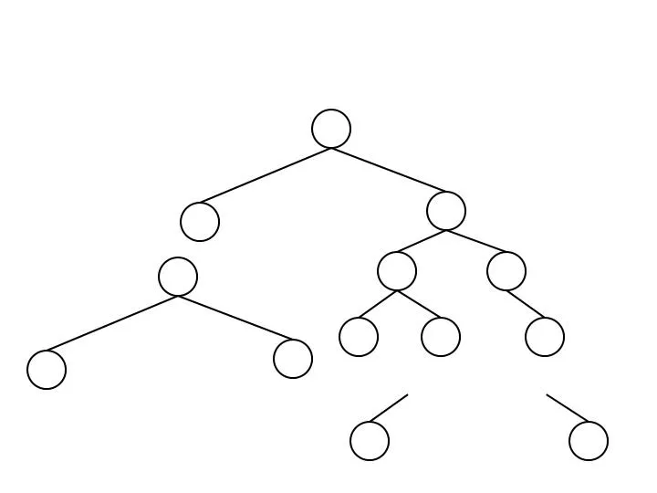
When dealing with obst • An optimal binary search tree is a binary search tree for which the nodes are arranged on levels such that the tree cost is minimum • In each binary tree there are NULL links at the leaf node, and they are denoted by square nodes • A tree with n nodes will have (n+1) NULL links
The square nodes are called as External nodes, b`coz`they are not a part of the tree • The inner round nodes are called as Internal nodes • Each time we search a element which is not in the tree the search ends at External nodes • Hence external nodes are also called as failure nodes • A tree with external nodes is called as extended binary tree
Extended binary trees Fig a Fig b 10 10 5 20 25 5 20 15 25 15
Path length affects the cost • Internal path length: - sum of path length of each internal node • External path length: - sum of path length of each external node
. L=0 Internal path length I=0+1+1+2+3=7 5 25 L=1 10 20 External path length E=2+2+2+3+4+4=17 L=2 15 L=3 E=I+2(no of nodes) Tree with max E will have max I L=4
If the user searches a particular key in the tree, 2 cases can occur: 1 – the key is found, so the corresponding weight ‘p’ is incremented; 2 – the key is not found, so the corresponding ‘q’value is incremented.
Cost of a bst when the searches are successful • Cost = Probability of node i Level of node i
Total cost • As we know that there is a possibility of both successful and unsuccessful searches • Cost= +
k2 k2 k1 k4 k1 k5 d0 d1 d0 d1 d5 k4 k3 k5 Figure (a) d2 d3 d4 d5 d4 k3 d2 d3 Figure (b)
We can calculate the expected search cost node by node: Cost= Probability * (Depth+1) Cost= Probability * (Depth+1)
And the total cost = (0.30 + 0.10 + 0.15 + 0.20 + 0.60 + 0.15 + 0.30 + 0.20 + 0.20 + 0.20 + 0.40 ) = 2.80 (Fig a) • So Figure (a)(complete bst) costs 2.80 ,on another, the Figure (b) costs 2.75, and that tree is really optimal.
k2 k1 k5 • We can see the height of (b) is more than (a) , and the key k5 has the greatest search probability of any key, yet the root of the OBST shown is k2.(The lowest expected cost of any BST with k5 at the root is 2.85) d0 d1 d5 k4 d4 k3 d2 d3 Figure (b)
So itz not necessary that always the key with highest probablityshould be the root
Property of an obst Sub tree Sub tree Sub tree Sub tree Optimal Optimal Optimal
To find the OBST, our idea is to decide its root, and also the root of each subtree •To help our discussion, we define : Ei,j = expected time searching keys in (k i ; d j) Real nodes from 1 - 5 dummy nodes from 0 - 5
Deciding Root of OBST • E[i,j] = minr { Ei,r-1 + Er+1,j + wi,j } Here r lies between i and j • Corollary: • Let r be the parameter that minimizes • { Ei,r-1 + Er+1,j + wi,j } • Then the root of the OBST for keys • ( ki, ki+1, …, kj; di-1, di, …, dj ) should be set to kr
Computing Ei,j Define a function Compute_E(i,j) as follows: Compute_E(i, j) /* Finding Ei,j */ 1. if (i == j+1) return qj; /* Exp time with key dj */ 2. min = 1; 3. for (r = i, i+1, …, j) { g = Compute_E(i,r-1) + Compute_E(r+1,j) + wi,j ; if (g <min) min = g; } 4. return min ;
Remarks •A slight change in the algorithm allows us to get the root of each subtree, and thus the structure of OBST (how?) •The powerful technique of storing computed is called Dynamic Programming •Knuth observed a further property so that we can compute OBST in O(n2) time (search wiki for more information)