Download

1 / 14
140 likes | 388 Vues
MACROECONOMIC EQUILIBRIUM AND FISCAL POLICY. Upon completing this lecture, students should understand the AD and AS model, Short-run and long-run equilibrium within the macroeconomy, and fiscal policy. Both the classical and Keynesian's point of view will be presented. OBJECTIVES

E N D
MACROECONOMIC EQUILIBRIUM AND FISCAL POLICY Upon completing this lecture, students should understand the AD and AS model, Short-run and long-run equilibrium within the macroeconomy, and fiscal policy. Both the classical and Keynesian's point of view will be presented. OBJECTIVES 1. Understand the AD and AS model. 2. Compare and contrast short-run and long-run equilibrium. 3. Illustrate and define business cycles. 3. Define multiplier and its applications. 4. Evaluate the effectiveness of changes in fiscal policy. TOPICS Please read all the following topics. AGGREGATE DEMAND AGGREGATE SUPPLY SHORT RUN AND LONG RUN EQUILIBRIUM BUSINESS CYCLES CLASSICAL AND KEYNESIAN ECONOMICS SELF-REGULATING ECONOMY AGGREGATE EXPENDITURE MODEL AN EXAMPLE FISCAL POLICY
Aggregate Demand The aggregate demand (AD) curve shows the real output (real GDP) that people are willing and able to buy at different price levels, ceteris paribus. The AD curve shows an inverse relationship between price level and domestic output (real GDP in billions). The explanation of the inverse relationship is not the same as for demand of a single product, which centered on substitution and income effect. The explanations are: 1. Wealth and real balances effect: when price level falls, purchasing power of existing financial assets rises, which can increase spending. People fell wealthier when price level falls and will be encouraged to buy more goods and services. 2. Interest-rate effect: when price level increases, businesses and households may have to borrow additional funds to complete their planned purchases. As borrowing demand increases, the interest rate rises, reducing actual borrowing amount and curtail planned consumption and investment. A decline in price level means lower interest rates which can increase certain spending. 3. Foreign purchases effect: when price level falls, other things being equal, US prices will fall relative to foreign prices, which will tend to increase spending on US exports and also decrease import spending in favor of US products that compete with imports. A change in the quantity demanded of Real GDP occurs because of a change in the price level. This causes a movement along the AD curve, but not a shift of the AD curve. A change in an economic variable other than price would be required to shift the AD curve. The economy consists of four sectors: Household, Business, Government, and foreign sector. Every sector buys a portion of GDP. The sum of their demand is called total expenditure (TE) or aggregate expenditure (AE). AE = C + I + G + Xn
Aggregate Demand Factors that change C, I, G, and Xn will change AE and AD. These factors are listed below: 1. Consumption: Wealth, interest rate, income taxes, and expectations about future prices and incomes will change C and shift AD curve. 2. Investment: Interest rate, business taxes, and expectation about future sales will change I and shift AD curve. 3. Foreign Sector: Foreign real national income and exchange rate will change export and import, causing AD curve to shift. 4. Money Supply: The money supply affects interest rates. An increase in money supply will lower interest rate, causing the AD curve to shift to the right.
Aggregate Supply (AS) curve below shows level of real domestic output (real GDP in billions) available at each possible price level, ceteris paribus. The upward slope of the curve indicates that producers are willing and able to sell more units of their goods as prices increase, and that their willingness to sell decreases as prices falls. The reasons listed below explaining the AS's upward sloping shape in the short run: Aggregate Supply 1. Rigid Wages: Economists believe that wages tend to be fixed by contracts or other agreements. When prices rise, but higher wages do not accompany them , producers' profits will rise temporarily, and the firm will produce more. 2. Sticky Prices: Prices are costly to change in some industries (menu costs). Where this is true, decreases in the general price level will negatively affect sales, profits, and output, causing producers to produce less. These two reasons given for the upward sloping AS are likely to be true only for short periods of time, and thus the AS curve described above is often called short run AS (SRAS) curve.
Aggregate Supply A change in the general price level will change the quantity supplied of the domestic output, this is a change along the AS curve. Other economic variables will change the SRAS curve and shift the curve to a new position. Some of these factors are listed below: 1. The Wage Rate: Higher wage rates means higher labor cost. Given constant prices, higher production costs reduce the profit per unit and lowering the number of goods produced. Therefore, higher wage rate shifts the SRAS curve to the left. 2. Prices of Non-labor inputs: Energy, land, capital and other non-labor inputs also have a significant impact on SRAS. An increase in the price of these inputs shifts the SRAS curve to the left. 3. Productivity: This is the output produced per unit of input used over a period of time. Higher productivity of labor or any other inputs will shift the SRAS to the right. 4. Supply Shock: Major natural or institutional changes will affect AS. Shocks like the Iraq War and 9/11 both impacted the AS. As mentioned earlier, factors created the upward sloping SRAS are not present in the long run. In the long run, the economy will always produce the full employment real GDP called potential GDP (GDPp) or natural real GDP ( Qn). The long run AS (LRAS) curve will be vertical at this real GDP level. Change in potential GDP will shift the LRAS curve to the right.
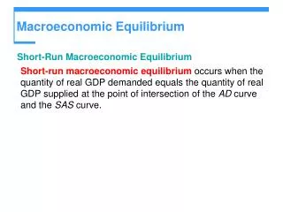
Equilibrium Short Run Equilibrium Putting AD and SRAS together, two curves will intercept at a point. This point is the short run equilibrium. This price level is the equilibrium price level, Pe; this quantity is the equilibrium quantity, Qe. At any other price level, the economy is either in surplus or in shortage. Long Run Equilibrium The interception point of AD and SRAS may be on the LRAS, creating a long run equilibrium where real GDP is equal to potential real GDP. If the potential GDP is at 600, then the following graph shows that the SR equilibrium is on the LRAS curve, creating a LR equilibrium. However, short-run equilibrium (real GDP) may occur on a level above or below the potential GDP, creating a disequilibrium in the economy.
GDP Gaps Recessionary gap If real GDP < Potential real GDP (full employment GDP), then a recessionary gap exist. At the same time: Unemployment rate > natural rate of unemployment. Since more job seekers are in the market, they tend to settle with a lower wage. Lower wage will increase the AS curve, causing the price to decrease. Lower price will increase consumption. This process will continue until the economy reaches the long run equilibrium (potential real GDP). If the potential GDP is at 700, graph on the right presented a recessionary gap between SR equilibrium and the LRAS curve. Inflationary gap If real GDP > Potential real GDP (full employment GDP), then an inflationary gap exist. At the same time: Unemployment rate < natural rate of unemployment. Since job seekers are less than job openings in the market, employers are forced to raise the wage to attract new workers. High wage will decrease the AS, and raise the price. Higher price will lower consumption. This process will repeat until the long run equilibrium is reached. If the potential GDP is at 500, left graph presented an inflationary gap between SR equilibrium and the LRAS curve.
Classical and Keynesian Economics CLASSICAL ECONOMICS According to Say’s law, supply creates its own demand. Excess income (savings) should be matched by an equal amount of investment by business. Interest rates, wages and prices should be flexible. The classical economists believe that the market is always clear because price would adjust through the interactions of supply and demand. Since the market is self-regulating, there is no need to intervene. Economists who advocate this approach to macroeconomic policy are said to advocate a laissez-faire approach. The market will reach full employment by itself. KEYNESIAN ECONOMICS The great depression is 1930s seemed to refute the classical idea that markets were self-correcting and should provide full employment. Keynes provided some explanations: 1) savings and investments are not always equal; 2) producers may lower output instead of prices to reduce inventories; 3) Lower production may increase unemployment rate and decrease incomes; 4) monopoly power on the part of producers and labor unions would prevent prices and wages to adjust downward freely. According to Keynes’ theory, wages and prices are not flexible. Rigid price will give a horizontal AS curve in the short run.
Self-Regulating Economy Classical economists believe in self-regulating economy. Wage rate and prices are flexible. Through the market mechanism, economy will move towards long run equilibrium. Recessionary gap If real GDP < Natural real GDP (full employment GDP), then a recessionary gap exist. At the same time: Unemployment rate > natural rate of unemployment. Since more job seekers are in the market, they tend to settle with a lower wage. Lower wage will raise the short run AS curve and causing the price to decrease. Lower price will increase consumption. This process will continue until the economy reaches the long run equilibrium (natural real GDP). Inflationary gap If real GDP > Natural real GDP (full employment GDP), then an inflationary gap exist. At the same time: Unemployment rate < natural rate of unemployment. Since job seekers are less than job openings in the market, employers are forced to raise the wage to attract new workers. High wage will decrease the short run AS, and raise the price. Higher price will lower consumption. This process will repeat until the long run equilibrium is reached.
Aggregate Expenditure Model Aggregate expenditure (AE)is the sum of consumption, investment, government purchases, and net export. Of these four sectors, the consumption represents the largest share. The consumption function: C = Co + MPC (Yd) C = total consumption Co = autonomous consumption whose amount is independent of disposable income MPC = marginal propensity to consume. This is a fraction between 0 and 1; and MPC is equal to change in consumption brought about by a change in disposable income. (MPC = change in C / change in Yd ) Yd = disposable income. A similar concept as MPC is MPS: marginal propensity to save. It is equal to change in savings (S) brought about by a change in disposable income. (MPS = change in S / change in Yd) Since all income must be either consumed or saved, then any change in income must also be consumed or saved. Therefore: MPC + MPS = 1 The average propensity to consume (APC) is the portion of income spent on consumption. (APC = C / Yd) The average propensity to save (APS) is the portion of income saved. (APS = S / Yd) Again, APC + APS = 1
Equilibrium GDP EQUILIBRIUM GDP Equilibrium GDP is the level of output whose production will create total spending just sufficient to purchase that output. If the economy produces an amount of goods that differs to the amount that the four sectors of the economy buy (AE), AE and aggregate production ( AP) are not equal; then the economy is in disequilibrium. When AE < AP, firms will involuntarily accumulate inventory. This will signal firms that they have overproduced. As a result, firms will cut back on production and/or prices. This will decrease the total value of output, moving the economy towards the equilibrium GDP. When AE > AP, inventories will be depleted unexpectedly. This will signal firms that they have not produced enough. As a result, firms will increase productions and/or prices. This will increase the total value of output, moving the economy towards the equilibrium GDP. MULTIPLIER Keynes observed that changes in autonomous expenditures (those expenditures independent of income) could create even larger changes in national income. For example, a technological break through has increased the autonomous investment by $50million, this $50M will become the income of the resources market. Workers who may have higher income are willing to spend more in the market. Their spending becomes the income of producers who will again spend in the market, and create extra income. This process repeats itself, creating a multiplier effect. If the Multiplier (M) = 2.5, then the aggregate expenditure will increase by $50M X 2.5 = $ 125M. M = 1 / MPS is commonly used to calculate the expenditure multiplier. An individual may increase the aggregate expenditure if he took $100 from his shoebox and spent on goods and services. His initial expenditure could be multiplied if the retailers who received the $100 spent part of the $100 to buy more supplies from the wholesalers, and the wholesalers might buy more from the manufacturers. This process continues to create a multiplier effect in the economy. The aggregate expenditure would be increased by a multiple amount. Obviously, if an individual took $100 and put into his shoebox, he would decrease the aggregate expenditure by a multiple of that amount.
An Example In this example, the equilibrium between AE and AP is illustrated. Data in this table is used to construct the graph below. As you can see from the graph in the next page, investment has increased the equilibrium GDP, (from the intersection of red and blue curves to the new intersection of red and yellow curves). The same equilibrium GDP can be obtained by observing the Investment and Saving schedule. In both graphs, we can see that equilibrium GDP is at 360. Another approach to get the equilibrium GDP is by using the multiplier. The equilibrium GDP, GDPe, before the investment is 260. MPC for this data set is 0.8. Multiplier = 1 / 1-MPC = 1 / (1-0.8) = 5 The investment amount of 20, will increase GDPe by 5 times, this will give us an increase of 20 X 5 = 100. Therefore, the new equilibrium GDP will be 260 + 100 = 360.
Fiscal Policy Government may change its expenditures and taxation to achieve particular macroeconomic goals. Fiscal policy is one of the most important economic tools available to the federal government. a. Expansionary fiscal policy: policy adopted during recession, aiming to increase AD through increases in government spending or decreases in taxes. b. Contractionary fiscal policy: policy adopted during inflation, aiming to decrease AD through decreases in government spending or increases in taxes. After the second quarter of 2001, the U.S. economy has entered into a recession phrase. In order to counter the recession, the Bush administration has started to impose the expansionary fiscal policy. Households got tax refunds. Government has increased expenditure in various sectors such as national defense (especially after September 11’s attack). The effect of expansionary or contractionary fiscal policy will be multiplied by the multiplier. For example, government has decided to provide a $40B aid for the airline industry after September 11, 2001. This $40B increase in government spending will increase the aggregate expenditure by $100B (for M = 2.5). However, the effect of fiscal policy is limited by certain factors: such as the crowding out effect, foreign loanable funds effect and time lag problems. Crowding out effect: Crowding out effect is quite important because it can completely erase fiscal policy's intention to correct the market. As the government tried to spend more to correct the recessionary gap in our economy, they compete with private sector for resources and goods and services. As government expenditure increases, consumption and investment decreases, causing the ineffectiveness of the fiscal policy. On the other hand, in the expansionary fiscal policy, government increases spending and reduces taxation, most likely result in a deficit which must be funded through borrowing. This increased borrowing will push the interest rate higher, reducing the consumption and investment in the private sector.