Macroeconomic Equilibrium
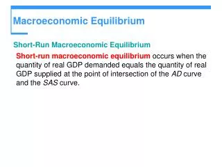
Macroeconomic Equilibrium. Short-Run Macroeconomic Equilibrium Short-run macroeconomic equilibrium occurs when the quantity of real GDP demanded equals the quantity of real GDP supplied at the point of intersection of the AD curve and the SAS curve. Macroeconomic Equilibrium.

Macroeconomic Equilibrium
E N D
Presentation Transcript
Macroeconomic Equilibrium • Short-Run Macroeconomic Equilibrium • Short-run macroeconomic equilibrium occurs when the quantity of real GDP demanded equals the quantity of real GDP supplied at the point of intersection of the AD curve and the SAS curve.
Macroeconomic Equilibrium • Short-Run Equilibrium • occurs at point c.
Macroeconomic Equilibrium • Long-Run Macroeconomic Equilibrium • Long-run macroeconomic equilibrium occurs when real GDP equals potential GDP—when the economy is on its LAS curve.
Macroeconomic Equilibrium Figure 23.9 illustrates long-run equilibrium. Long-run equilibrium occurs where the AD and LAS curves intersect and results when the money wage has adjusted to put the SAS curve through the long-run equilibrium point.
Macroeconomic Equilibrium • Economic Growth and Inflation • Figure 23.10 illustrates economic growth and inflation.
Macroeconomic Equilibrium • Economic Growth and Inflation • Economic growth occurs because the quantity of labor grows, capital is accumulated, and technology advances, all of which increase potential GDP and bring a rightward shift of the LAS curve.
Macroeconomic Equilibrium • Economic Growth and Inflation • Inflation occurs because the quantity of money grows faster than potential GDP, which increases aggregate demand by more than long-run aggregate supply. • The AD curve shifts rightward faster than the rightward shift of the LAS curve.
Macroeconomic Equilibrium • The Business Cycle • The business cycle occurs because aggregate demand and the short-run aggregate supply fluctuate but the money wage does not change rapidly enough to keep real GDP at potential GDP.
Macroeconomic Equilibrium • A below full-employment equilibrium is an equilibrium in which potential GDP exceeds real GDP. • Figures 21.11(a) and (d) illustrate below full-employment equilibrium. • The amount by which potential GDP exceeds real GDP is called a recessionary gap.
Macroeconomic Equilibrium • A long-run equilibrium is an equilibrium in which potential GDP equals real GDP. • Figures 21.11(b) and (d) illustrate long-run equilibrium.
Macroeconomic Equilibrium • An above full-employment equilibrium is an equilibrium in which real GDP exceeds potential GDP. • Figures 21.11(c) and (d) illustrate above full-employment equilibrium. • The amount by which real GDP exceeds potential GDP is called an inflationary gap.
Macroeconomic Equilibrium • Figure 23.11(d) shows how, as the economy moves from one type of short-run equilibrium to another, real GDP fluctuates around potential GDP in a business cycle.
Macroeconomic Equilibrium • Fluctuations in Aggregate Demand • Figure 23.12 shows the effects of an increase in aggregate demand. • Part (a) shows the short-run effects. • Starting at long-run equilibrium, an increase in aggregate demand shifts the AD curve rightward.
Macroeconomic Equilibrium • Fluctuations in Aggregate Demand • Firms increase production and rise prices—a movement along the SAS curve.
Macroeconomic Equilibrium • Fluctuations in Aggregate Demand • Figure 23.12(b) shows the long-run effects. • Real GDP increases, the price level rises, and in the new short-run equilibrium, there is an inflationary gap.
Macroeconomic Equilibrium • Fluctuations in Aggregate Demand • The money wage rate begins to rise and short-run aggregate supply begins to decrease. • The SAS curve shifts leftward. • The price level rises and real GDP decreases until it has returned to potential GDP.
Macroeconomic Equilibrium • Fluctuations in Aggregate Supply • Figure 23.13 shows the effects of a decrease in aggregate supply. • Starting at long-run equilibrium, a rise in the price of oil decreases short-run aggregate supply and the SAS curve shifts leftward.
Macroeconomic Equilibrium • Fluctuations in Aggregate Supply • Real GDP decreases and the price level rises. • The combination of recession combined with inflation is called stagflation.
U.S. Economic Growth, Inflation, and Cycles • Figure 23.14 interprets the changes in real GDP and the price level each year from 1963 to 2003 in terms of shifting AD, SAS, and LAS curves.
U.S. Economic Growth, Inflation, and Cycles • From1963 to 2003: • Real GDP and potential GDP grew from $2.8 trillion to $10.3 trillion. • The price level rose from 22 to 105. • Business cycle expansions alternated with recessions.
U.S. Economic Growth, Inflation, and Cycles • Economic Growth • Real GDP growth was rapid during the 1960s and 1990s and slower during the 1970s and 1980s. • Inflation • Inflation was the most rapid during the 1970s. • Business Cycles • Recessions occurred during the mid-1970s, 1982, 1991–1992, and 2001.