Faults I
Faults I. Fault. A fault is a mesoscopic to macroscopic plane ( listric faults are curved at large scale !) along which the two blocks on either side have displaced (slipped) relative to one another The slip is primarily due to brittle deformation

Faults I
E N D
Presentation Transcript
Fault • A fault is a mesoscopic to macroscopic plane (listric faults are curved at large scale!) along which the two blocks on either side have displaced (slipped) relative to one another • The slip is primarily due to brittle deformation • This distinguishes faults from fault/shear zone • Deformation in a fault zone is distributed along a set of closely-spaced faults within a zone • Deformation in a shear zone is ductile (i.e., high strain without macroscopic loss of cohesion), involving either crystal plastic or catraclastic flow mechanisms (or a combination = semibrittle)
Scale of Faults • The range of size for faults is from: • microscopic, mm scale (10-3 m), to • thousands of kilometer (106 m) • (regional, lithospheric) • A fault is called a shear fracture if its dimensions are smaller than one meter
Net Slip • The net slip of a fault is the magnitude and direction of relative displacement on the fault plane between two previously contiguous points (piercing points). • The net slip is a vector; it requires magnitude (e.g., in meters) and a direction (trend/plunge) • It can be resolved into its components • We also need to define the sense of slip (or shear) to completely define the net slip
Net slip • The net slip vector can be resolved into any arbitrary pair of components, for example • along the strike (strike-slip) • along the dip (dip-slip) • oblique to the strike (oblique-slip) • This is the most common case! • The components for the dip-slip are: • Heave: horizontal component of dip-slip • Throw: vertical component of dip-slip
Measuring Net Slip • Need two previously contiguous points (piercing points) on the fault plane • These two points (one on the hanging wall and the other on the footwall) are the intersection of a so-called piercing line with the fault • The piercing line, defined by intersection of two planes (e.g., two beddings, fault and bedding), becomes broken after faulting
Slip Lineation • Lineation on the fault plane that form parallel to the net slip, for at least the last increment of slip • Slip lineation forms parallel to the intersection of the fault plane and the movement plane (M-plane, which is the 13 plane) • The 13 plane, of course, is perpendicular to the 2, which lies on the plane of the fault(s) • It also contains the pole to the fault • The M-plane is constructed by putting the pole to the fault and the slip lineation on a same great circle • The attitude of the slip lineation provides the attitude of latest slip (trend/plunge) • The sense of slip may be provided with shear indicators on the fault surface
Anderson Faulting Theory • The surface of Earth is a principal plane of stress (i.e., there is no shear stress along the surface of Earth) • The normal to the surface is therefore parallel to one of the principal stresses (1, 2, 3)
Principal stresses and faults • According to the Anderson theory of faulting, one principal axis of stress is always perpendicular to the earth surface (i.e., is vertical), while the other two are horizontal • Normal fault: 1 is vertical • Reverse fault: 3 is vertical • Strike-slip fault: 2 is vertical
Terminology - Non-vertical faults • Block above the fault plane is the hanging-wall • Block below the fault plane is the footwall • By convention, geologist keep track of the movement of the hanging wall (not the footwall) • The hanging wall can move up or down • This is the basis of the classification of faults
Plots of slip lineation for kinematic analysis • These plots (of slip linear) are used for kinematic analysis, i.e., determining the direction of motion along the fault • For this we need the attitude of the fault, the orientation of the slip lines, and the sense of slip • In this plot, the slip line is decorated with an arrow which indicates the direction (and sense) of slip (along the M-Plane)
Procedure for plotting fault data • Plot the trace of the fault and its pole • If there are two conjugate faults, then plot bothNote: • The conjugate faults develop if the difference in the value between the maximum and the other two principal stresses is significant • If the intermediate and minimum principal stresses are equal, and say 1 is vertical, then normal faults with variable strikes would develop. • For each fault, plot the slip lineation (using its trend/plunge or pitch) on the fault plane
The intersection of the two conjugate faults defines the direction of the 2 • The bisector of the acute angle defines the1, and the bisector of the obtuse angle defines the 3 • Both 1 and 3 lie on the M-Plane • Plot the M-plane (it contains the fault pole and slip line) • Decorate the slip line, on the M-plane/fault, with a short line (called ‘slip linear’), drawn along the M-plane • If we know the sense of slip (e.g., normal, reverse), say from slip fibers, decorate the line with an arrow to indicate the relative movement of the HW block (e.g., arrow points updip along the M-plane) • Distinguish the upward slip lines from downward ones
Fault-slip data collected at selected sites along the main transverse faults in the Northern Apennines. Bonini, 2009
Notice that the direction of the 1 should be steep for the case of normal faults, and the slip linear(s) must be along the true dip, downdip toward the premitive • For the case of a reverse fault, 1 should be gently plunging, near the primitive, and the slip linear(s) should point updip • For the case of strike slip fault, 1 is near the primitive, and the sense of the slip is indicated by a couple (remember that the acute wedge facing 1 goes in!). • For each case, conjugate faults intersect along the 2
Direction of shortening vs. extension • From the slip linear and fault’s orientation, we can find the shortening and extension axes for the fault These axes lie on the M-plane • They are perpendicular to each other • The slip linear arrow points toward the extension axis, and away from the shortening direction
A set of conjugate normal faults, with slip lines and slip linears. The corresponding M-planes and M-axes (normal to the M-planes). http://docvsoft.com/orient/Documentation/html/ch03_spherical.html
Tension axes or T-axes (yellow) and pressure axes or P-axes (green) for the same data set on last slide, with a contoured gradient on the P-axes. A beach ball diagram, can be plotted to display the fault nodal planes. The nodal planes are estimated based on the eigenvectors of the M-axes and P-axes. http://docvsoft.com/orient/Documentation/html/ch03_spherical.html
Differential stress and faulting • In sandbox experiments, it has been shown that: • Normal faults form when 1 remains constant while 3 weakens (i.e., differential stress increases as 3 goes to the left on the Mohr diagram) • i.e., vertical push is constant, while 3 (horizontal) is reduced, i.e., circle grows to the left • Reverse faults form when 3 remains constant while increases 1 increases • i.e., circle grows to the right on the Mohr diagram
Terminology • Emergent fault • Active fault that cuts the surface of Earth • Exhumed fault • Exposure of an inactive fault at the surface due to uplift or erosion • Blind fault • A fault that dies out in the subsurface without intersecting the surface of Earth
General Types of Fault • Faults are divided into the following three categories based on the relative displacement of the fault blocks with respect to the attitude of the fault plane: • Dip slip fault - The hanging wall block moves (up or down) parallel to the dip of the fault plane • The net slip is pure dip-slip
Classification of Faults … • Strike slip fault - Both blocks move parallel to the strike of the fault plane • There is no hanging wall in this case! • The net slip is pure strike-slip • Oblique slip fault - The displacement vector is oblique to both strike and dip • The senses of both the dip slip (normal or reverse) and strike slip (left- or right-lateral) are needed for a oblique-slip fault • Left-lateral, normal, oblique-slip fault • Right-lateral, reverse, oblique-slip fault
Extensional or Contractional • Contractional fault • Forms due to shortening of the layers • Rock units become duplicated • Includes reverse and thrust fault • Extensional fault • Forms due to lengthening of a layer • Involves loss of stratigraphic section • Includes normal fault
Dip-slip Faults • Dip-slip - Motion is along the dip • High-angle ( >60o) • Intermediate angle (30o-60o) • Low-angle <30o) • Two types of dip-slip: Normal and Reverse • Normal fault - If the relative motion of the hanging wall block is down-dip on the fault • Is caused by extension • Forms horst and graben • Example: Basin and Range, Mid-ocean ridge
Dip-slip Faults • Reverse fault, if the motion of the hanging wall block is up-dip on the fault. • Caused by contraction • e.g., faults in subduction zones • Thrust is a low-angle reverse fault • e.g. Grand Tetons; the Appalachians
Strike-slip Faults • Strike-slip - one block moves horizontally past another block: • Are usually very long (100’s - 1000’s of km) • NOTE: • At a small scale, fault attitude may be constant • At a larger scale, however, both the dip and/or strike of a fault may change
Strike-Slip Faults - Types • Left-lateral (sinistral) strike slip fault • To an observer standing on one block and looking across the fault, the other block seems to have moved to the left • Right-lateral (dextral) strike slip fault • The block across the fault moved to the right of the observer. e.g., San Andreas fault • Oblique-slip • motion is oblique to dip and strike • e.g., normal, left-lateral, right-lateral, reverse
Fault Type • Listric fault: • The dip of the fault varies with depth. • Fault bend: • Is where both the dip and strike of a fault changes. • Flat: • A fault which is locally parallel to the bedding (in the hanging wall or the footwall). • A fault parallel to bedding in the hanging wall may be across the bedding in the footwall, and vice versa! • Ramp: A fault which is locally across bedding
Bends • The change in the attitude of the fault steps the fault either to the left (left-step) or to the right (right-step) • Depending on the sense of displacement of the fault, the right or left step may produces either contraction (restraining bends) or extension (releasing bends) across the step
Basement thrust over younger sediments in transpressional segment of San Andreas fault
Fault Separation • Distance between the displaced parts of a marker as measured along a specific line, on a specific plane. • Is usually not the same as the net slip, unless the specified line is parallel to the net slip. • It depends on the attitude of the displaced marker. • NOTE: • Two non-parallel markers will produce different separation • Separation along the fault for one marker may show right-lateral, and for another, a left-lateral sense of slip!
Fault Separation - Facts • A strike-slip fault cutting a horizontal sequence of layers produces no horizontal (strike) separation! • A dip-slip fault cutting vertical layers produces no dip separation • Use linear features (e.g., fence, roads, etc.), or trace of a planar feature, on a horizontal plane, to determine the horizontal separation • Heave and throw are components of the dip separation
Faulting • Faulting, as a mode of failure, is the most significant way in which lithospheric masses are tectonically transported relative to each other, especially in the seismogenic upper crust • Deformation in this brittle part of the crust takes place by pressure-sensitive, strain rate-insensitive frictional sliding on discrete fault planes with little inelastic strain and dislocation activity • Faults commonly involve frictional sliding along pre-existing joints, veins, and other discontinuities, but can also initiate and propagate in intact rocks
Fault Geomorphology & Scale • Active faults such as the San Andreas: • Show considerable variation in the irregularity of their trace • Commonly occur in variably-oriented strands or segments • The segments grow and link as the total displacement increases • Range in fault length is over eight orders of magnitude (10-3 m to 105 m) • Display a power law size distribution; i.e., fractal
Fault Surface Structures • Fault displacement produces friction-related striations (polishing and grooving) indicating the latest, local direction of movement and sometimes absolute direction of movement • The slip lineation are called slickensides or slickenlines • Fiber growth in the direction of fault displacement, on the slickensided surface, provide clear indications of relative offset • Extensional fractures occur at a high angle to slip direction and dip steeply into fault plane
Structural features to Recognize Faults • polishing and grooving • slickensides • breccia • gouge • mylonite • shear zone • associated fractures • drag of layers adjacent to fault • juxtaposition of dissimilar rock types • displacement of planar structures
Geomorphic features • fault scarp • fault-line scarps • triangular facets • alignment of facets • increase of stream gradients at the fault line • hanging valleys • aligned springs and vegetation • landslides • displaced stream courses
Fault and Stress • Conjugate shear fractures develop at about = 30 degrees from 1 • 1 bisects the acute angle of about 60o between the two fractures • 3 bisects the obtuse angle between the two fractures
Faults and the Principal Stresses • Reverse faults are more likely to form if 3 is vertical and constant (at a standard state), while horizontal, compressive 1 and2 increase in value compared to the standard state • Normal faults form if 1 is vertical and constant, while horizontal 3 and2 decrease in value, or if horizontal 3 is tensile • Strike-slip faults form if 2 is vertical and constant, while horizontal 1 and2 increase and decreases in value, respectively